
In the first post in this series we saw how to run autoregressive model OLS in R, and calculate forecasted periods in Essbase based on OLS coefficients. We also saw how to generate predictions of future periods using ARIMA model, and load forecasted values back to Essbase.
Here we are going to use regressions and ODM to calculate a subset of accounts based on the known values of other accounts. The potential use case would be when the analyst manually updates forecasted accounts that are linked to future business activity. Values of those accounts cannot be forecasted with autoregressive models because, for example, there is some internal knowledge about the future that is not embedded in the past. For example, decision to go live with a new product, which will bring expenses in certain areas to a new level. Or assumptions about competitor’s behavior which will lead to changes in revenue or will change prices of raw materials.
So when we generate forecast, a subset of accounts will be updated manually (those accounts will reflect changes in business activity) - let’s call them drivers, whereas another subset that correlates strongly with the drivers, can be calculated using regressions. At the same time there could be accounts such as G&A, that may not be affected by the drivers, but are better forecasted by the autoregressive models.
But how can we choose those subsets? In some cases you have a pretty good idea about relationships between accounts. In the trivial case that could be a deterministic relationship. In some other cases you know that the relationship exists, but don’t know exact coefficients, whether the function describing the relationship is linear, logarithmic, polynomial, etc. And in some cases you are not even aware of a relationship.
Dynamic Pivoting of Accounts
Let's start with a basic form of linear regression. Suppose you have a strong feeling that Airfare and Travel Agency Fee accounts must be related, and you can predict Travel Fees with Airfare. You know that your air travel next year is going to increase since because of a new service launched globally. As a first step we need those 2 accounts in columns. The way we usually have data for Account dimension in staging areas or data marts that serve Essbase/Planning applications - accounts are in rows. When we export data from Essbase we have one column per dimension and 13 columns for periods, in case of monthly data. When we load data from ERP system we typically have a single data column.To make the data source available for running regressions we need to pivot accounts. For that purpose we can use PIVOT function. If we had only 3 accounts the query would look like this:
with t1 as (
select * from (
SELECT BUSINESSUNIT,
ENTITY,
PCC,
COSTCENTER,
SCENARIO,
VERSION,
YEAR,
HSP_RATES,
CURRENCY,
MNUM,
DATA,
ACCOUNT
FROM T_EPMA_FACT )
PIVOT (sum(DATA) as ACC FOR (ACCOUNT) IN
('12345' as "12345",'12346' as "12346",12347 as "12347"))
)
select "BUSINESSUNIT","ENTITY","PCC","COSTCENTER","SCENARIO"
,"VERSION","YEAR","HSP_RATES","CURRENCY","MNUM",
"12345_ACC","12346_ACC","12347_ACC"
from t1
WHERE 1=1 AND (nvl("12345_ACC",0)<>0 OR nvl("12346_ACC",0)<>0 OR nvl("12347_ACC",0)<>0 )
|
The problem though we may have hundreds of accounts, and some of them get added on a daily basis. Also the list of accounts in PIVOT function cannot be a subquery.
As a workaround we can dynamically generate a view with a stored procedure. The procedure will create a dynamic SQL statement based on the accounts currently existing in the data source. So even if new accounts were added into the source, it would be reflected in the view once we ran a stored procedure. Here’s a code for it:
create or replace PROCEDURE "PIVOTACCOUNT"
as
--DECLARE
TYPE cur_TYPE IS REF CURSOR;
FLEX VARCHAR2(200);
DESCFIELD VARCHAR2(200);
SQLSTMT CLOB;
SQLSTMT2 CLOB;
SQLSTMT3 CLOB;
excl_cursor cur_TYPE;
BEGIN
OPEN excl_cursor FOR
select distinct ACCOUNT from T_EPMA_FACT;
SQLSTMT:='CREATE OR REPLACE VIEW V_FACT_PIVOT_ACCOUNT AS
with t1 as (
select * from (
SELECT BUSINESSUNIT,
ENTITY,
PCC,
COSTCENTER,
SCENARIO,
VERSION,
YEAR,
HSP_RATES,
CURRENCY,
MNUM,
DATA,
ACCOUNT
FROM T_EPMA_FACT )
PIVOT (sum(DATA) as ACC FOR (ACCOUNT) IN (ACCOUNTPIVOTTOKEN))
)
select * from t1 WHERETOKEN
';
SQLSTMT2:='';
SQLSTMT3:='WHERE 1=1 AND (';
LOOP
FETCH excl_cursor INTO FLEX ;
EXIT WHEN excl_cursor%NOTFOUND;
SELECT SQLSTMT2||''''||FLEX||''' as "'||FLEX||'",' INTO SQLSTMT2 FROM DUAL;
SELECT SQLSTMT3||'NVL("'||FLEX||'_ACC",0)<>0) OR ' INTO SQLSTMT3 FROM DUAL;
END LOOP;
CLOSE excl_cursor;
SELECT SUBSTR(SQLSTMT2,0,LENGTH(SQLSTMT2)-1) INTO SQLSTMT2 FROM DUAL;
SELECT SUBSTR(SQLSTMT3,0,LENGTH(SQLSTMT3)-3)||')' INTO SQLSTMT3 FROM DUAL;
SELECT replace(SQLSTMT,'ACCOUNTPIVOTTOKEN',SQLSTMT2) INTO SQLSTMT FROM DUAL;
SELECT replace(SQLSTMT,'WHERETOKEN',SQLSTMT3) INTO SQLSTMT FROM DUAL;
dbms_output.put_line(SQLSTMT);
EXECUTE IMMEDIATE SQLSTMT;
END;
|
ACCOUNTPIVOTTOKEN and WHERETOKEN in the SQL statement are replaced with the list of accounts and WHERE clauses within the cursor.
Since running this view on a large table will take some time it’s probably a good idea to insert the output into a table before we start running multiple regressions on it.
Basic Linear Regression
Now let's build a simple workflow in order to run our regression. It consists of a SQL Query node and regression model.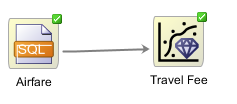
The query would be:
SELECT
"BUSINESSUNIT"||
"COSTCENTER"||
"CURRENCY"||
"ENTITY"||
"MNUM"||
"PCC"||
"YEAR" CASE_ID,
BUSINESSUNIT,
ENTITY,
PCC,
COSTCENTER,
SCENARIO,
VERSION,
YEAR,
HSP_RATES,
CURRENCY,
MNUM,
"12345_ACC",
"12346_ACC"
FROM T_FACT_PIVOT_ACCOUNT
where 1=1
and "12345_ACC" is not null
and "12346_ACC" is not null
|
Like in the previous examples of clustering we concatenate all level-0 members to generate CASE_ID. Target account is 12346_ACC (Travel Fees). First let’s try to run regression on Cost Center, Business Unit, Entity, PCC being independent variables, just as 12345_ACC. In general, the purpose of regression is to explain the variability of the dependent variable with the variability of independent variables. In case of other accounts - that’s a clear statement. But what about members of Cost Center dimension for example? Essentially each level-0 member becomes an independent dummy variable with only 2 possible values - 0 or 1.
Let’s say we want to use a single member (C_1234 ) of Cost Center dimension in regression. Hence we can write the formula as:
12346_ACC = intercept + Coeff1*12345_ACC+Coeff2*C_1234 + error
Whereas C_1234=1 if the observation belongs to C_1234, or 0 otherwise.
So if Coeff2=1000, then we know that on average our Travel fees are $1000 higher in C_1234 cost center.
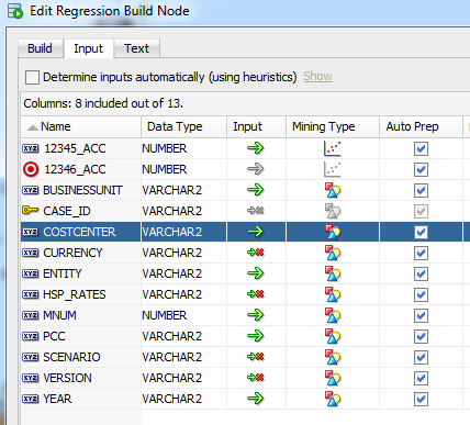
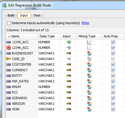
The input columns would look like this:
Now let’s review the results. Wald Chi-square and Pr>Chi-Square give you an indication how meaningful particular independent variable is. In other words - “These are the test statistics and p-values, respectively, for the hypothesis test that an individual predictor's regression coefficient is zero given the rest of the predictors are in the model.” So we should consider in our forecasts those independent variables that have higher ABS(Wald Chi-Square) and lower PR>CHi-Square (usually below 0.05).
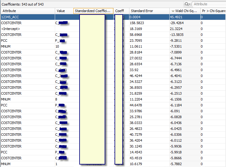
You can see that in addition to 12345_ACC (Airfare) there are multiple members that have very low Pr > Chi-Square. An interesting fact also is that coefficients of all MNUM values (month number dimension) are also non-zero. So we should probably consider time series predictors in addition to other accounts being predictors from the same period.
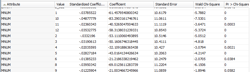
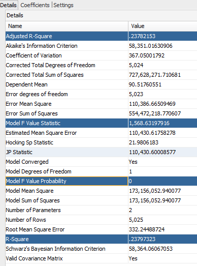
Let’s take a look at the regression details:
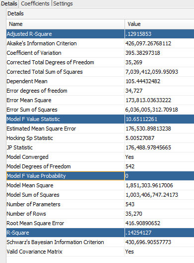
And finally Model F Value probability is 0, meaning that you can reject the null-hypothesis and conclude that the model provides a better fit than the intercept-only model, with probability of 100% (approximation obviously).
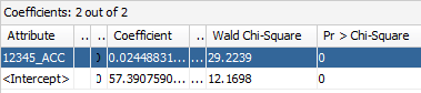
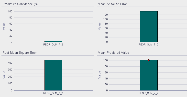
What if we remove dimensions from regression inputs, and leave only 12345_ACC (airfare) account as independent variable?
This would give us only 2 coefficients obviously:
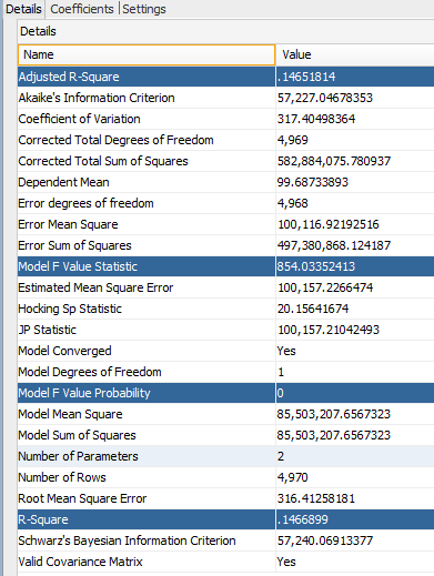
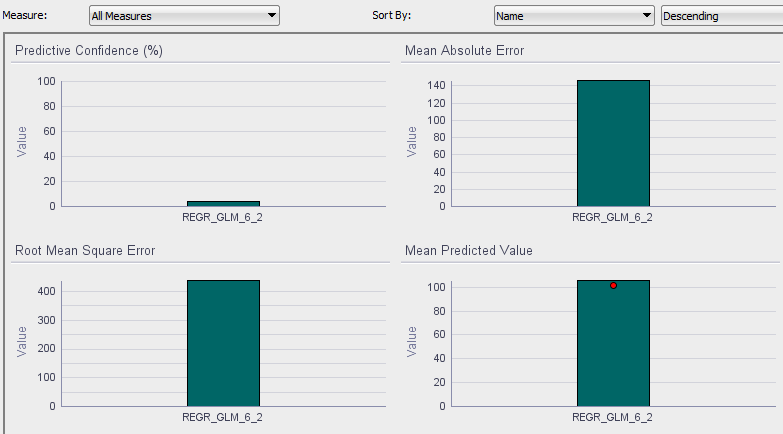
We can also review test results of these 2 models. REGR_GLM_6_2 is a model with dimensions, whereas REGR_GLM_7_2 with only Airfare independent account.
Using Cluster Information In Regressions
The next experiment we’d like to run is using specific cluster to filter the data source for the regression. Let’s use the clustering model we worked with in the last post. We’ll use leaf clusters: 2,4,6,...18.19.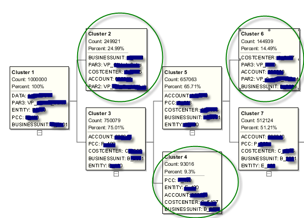
To filter the source data based on the cluster we can use cluster rule. Then we can add row filter node from transform components:
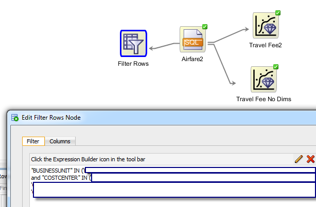
And finally add a new regression node and connect it with “Filter Rows” node. If we wanted to run a separate regression on each cluster and manually create the workflow we would end up with something like this:
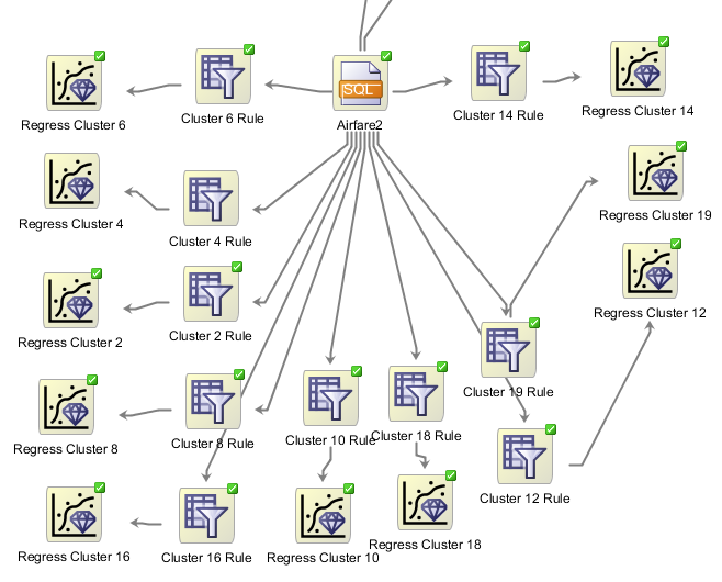
Given that clustering and using cluster rules is an iterative process, creating these workflows manually is hardly a viable option on a large scale. But we’ll see how to automate this in one of the next posts.
As far as the regression results here’s what we have for cluster 6:
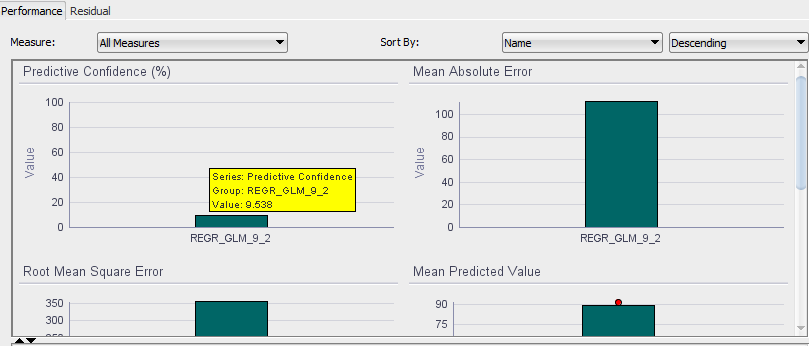
We have a much better predictive confidence of 9.5% (still pretty low, but improvement of ~300% nonetheless), and a better Adjusted R-Square:
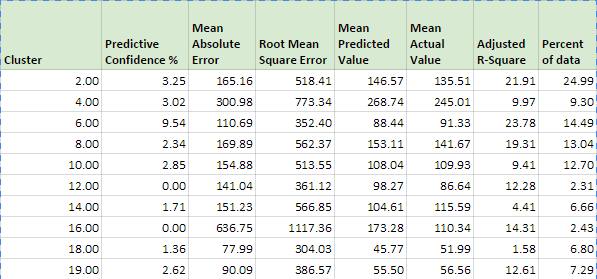
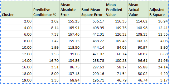
Below is a table describing regression results for the rest of the clusters. Clearly results are very different from regression when it was run on entire dataset. Although there are 3 clusters with higher Adjusted R-Square than the baseline, there’s only one cluster with higher predictive confidence.

What about other clustering methods? If we use clustering without upper level members of Cost Center dimension, we get quite different results:

Most of the clusters achieve better results than the baseline. This is true for both Adjusted R-Square and Predictive Confidence. Below is a chart showing predictive confidence of 2 clustering methods:

So, we can make 2 conclusions:
- With clustering we can achieve much better regression results than without clustering.
- Different clustering methods can have very different results in terms of predictive confidence or Adjusted R-Square and other performance metrics.
No comments:
Post a Comment