Descriptive Statistics And Clustering With Data Miner

Ok, this is my third post in a series of predictive analytics for Essbase/Planning. 

1. In the first one, “Essbase Meets R”, I described options to integrate Essbase with open source software R.
2. In the second, Essbase Meets R: Next Steps: ODM And ORE, we walk through steps to configure Oracle Data Miner (ODM) and Oracle R Enterprise (ORE).
3. Here we’ll see how to use descriptive statistics and run clustering models in ODM. Results of the clustering will be used by the forecasting models, and will be covered in the next posts.

First, let me say this is not supposed to teach you math/statistics. This is simply me playing with ODM and a demonstration how you could use various models. They may or may not be suitable for your particular problem. Consult with a statistician or a data scientist if you consider using them. 

Descriptive Statistics

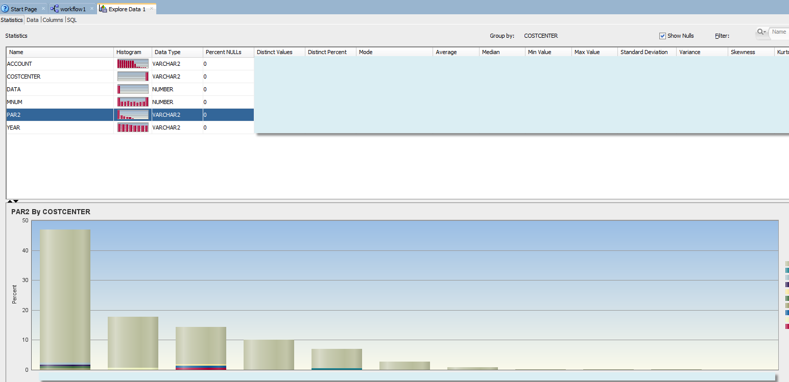
In the previous post we saw how to create a basic workflow that consists of a data source and "Explore" node.
Once we ran the workflow we can right click Explore Data node and select “View Data”. There we can see some nice histograms by dimension.



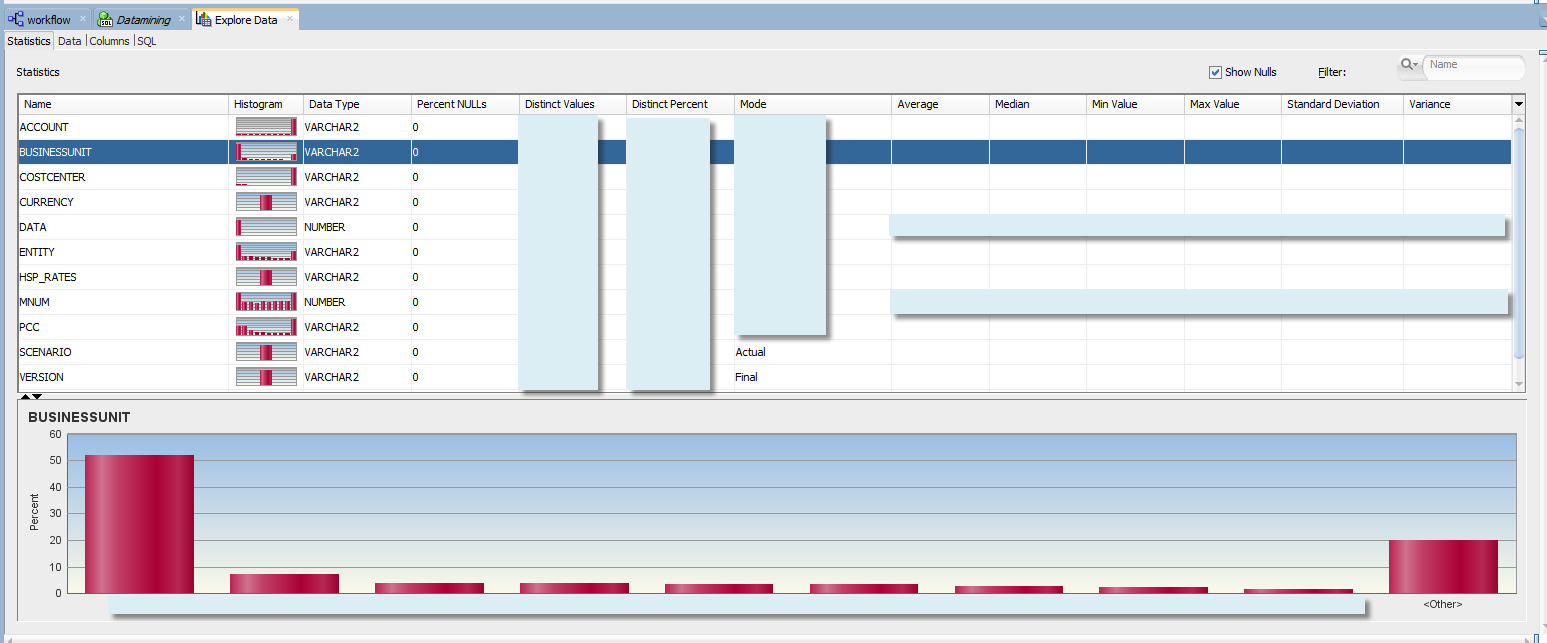
Histograms are especially useful when we just start examining our data. We can see how it is distributed across attributes (or dimension members in other words). In “Essbase Meets R” we tried to identify optimal sample dimensionality, or how to choose the appropriate levels from our hierarchies. When we run our model, we don’t want to mix up samples that behave completely differently (like Travel Expense of Sales cost centers and IT cost centers).

Histograms can be helpful in that respect, although in the next sections we’ll review more accurate methods, such as clustering and association rules.

At the first glance we can see that for some dimensions like BusinessUnit or Entity the data is concentrated in just a handful of members. 

Different data density is also an indication of different underlying business processes, relationships between the variables, and different distribution of the forecasted accounts. 



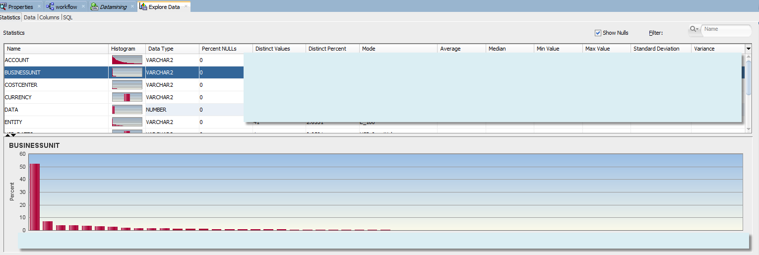
What if we change the number of bins from the default 10 to 100? In case of the Business Units we still have most of the data concentrated in a single member. 

But in case of the Cost Centers we have a different picture:

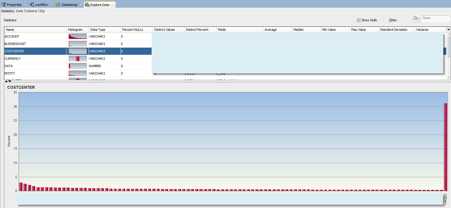
This means the data is distributed more evenly across cost centers. Does it mean we can combine all samples of individual cost centers? Not necessarily.  So far we were referring to level-0 and top node of the dimension. We don’t have dimensional information in this fact table. It contains only level 0 members of the hierarchy. Dimensional structures are stored in a separate table, and each dimension has an associated view. At least in this example. What if we wanted to examine histograms that include certain levels of cost center hierarchy? For example we want to see how level-0 cost centers are distributed within the 3rd generation of Cost Center dimension, or withing VP groupings of the hierarchy?

For that purpose we can create a view that will join a fact table with dimension view and will return data points with CostCenter ancestors - specifically the third generation member from the cost center hierarchy. And let's add that ancestor as an attribute of “Explore Data” step.

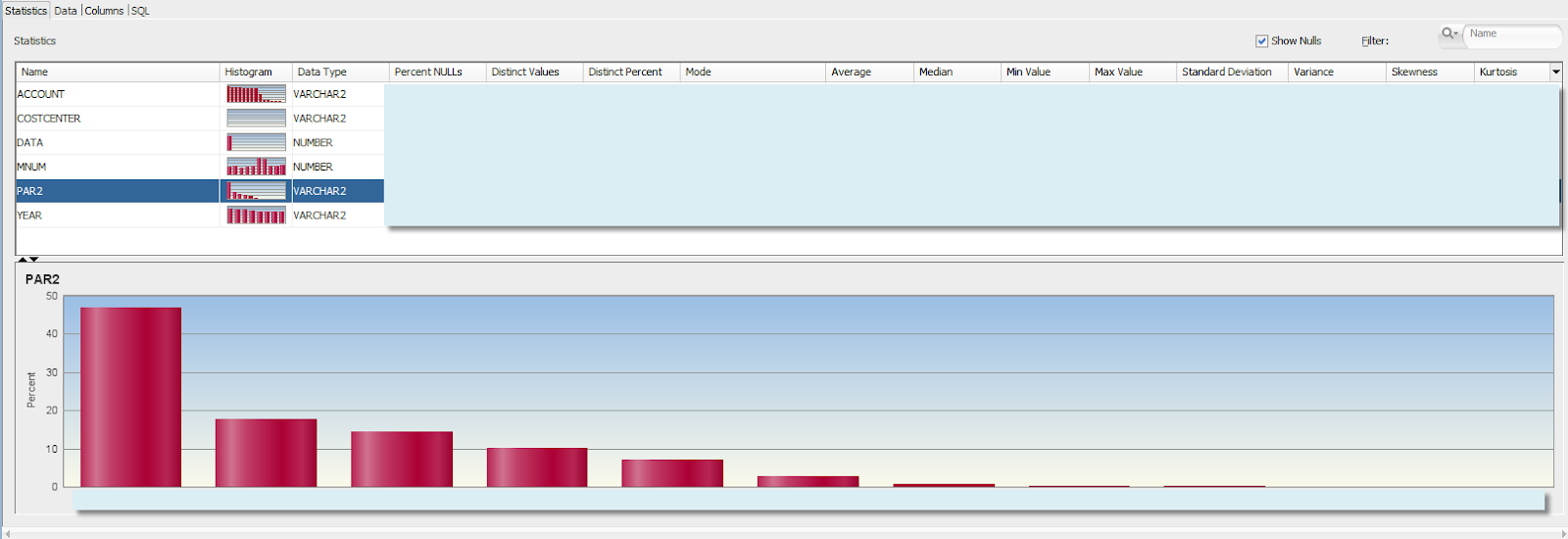
We can see that the data is concentrated differently in different VP cost centers. But does different data concentration necessarily mean that it is distributed differently as well (has different relationships between the variables)? The answer is no. You may simply have a different number of child cost centers under each parent, but the data in each child could be distributed similarly. We would need to take into account the number of children in each upper level cost center. 

Somewhat better picture of the data would be given by histogram with groupings by  level-0 cost centers. You can immediately see that some level-0 cost centers have different data concentration, as part of upper level VP cost centers. 

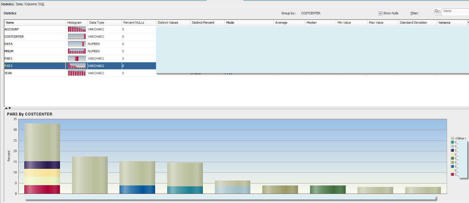
At this point we cannot really identify specific hierarchy level or subcubes in multidimensional space that should be used to combine samples. We can probably say our models should not be run neither for level-0 cost centers nor  for combined sample of all cost centers, and that we need to run additional analysis.

Another problem with this approach is that if you are planning to investigate histograms of many dimension-generation combinations, that’s a lot of nodes in the workflow, and a lot of manual work. 

The bottom line - “Explore Data” node of Oracle Data Miner can be useful for a quick data exploration, easy to use, and will give a quick insight about the data to the business user. But it would be hardly sufficient to support exploration across multiple levels of multiple dimensions in a systematic and repeatable way. That’s where clustering models come into picture. 

Clustering Models

First,  what exactly clustering models are? I’ll refer to Wiki for definition:

Cluster analysis or clustering is the task of grouping a set of objects in such a way that objects in the same group (called a cluster) are more similar (in some sense or another) to each other than to those in other groups (clusters). It is a main task of exploratory data mining, and a common technique for statistical data analysis, used in many fields, including machine learning, pattern recognition, image analysis, information retrieval, bioinformatics, data compression, and computer graphics.

ODM provides 3 clustering algorithms: K-Means, O-Cluster, and Expectation Maximization. As a first step let's consider clustering of our raw level-0 data. That is when we select all attributes from the fact table. 

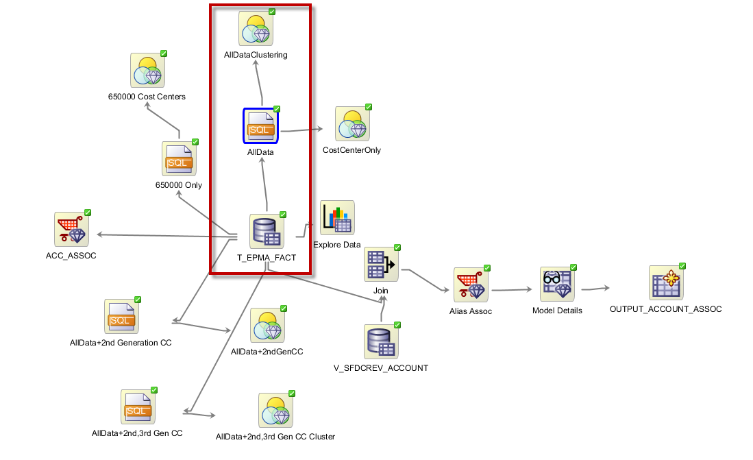
The outlined part of the demo workflow has query node that selects columns from data source node. It also contains CASE_ID column which is a concatenation of all level-0 members. This unique Case_ID is needed to run the clustering model. 

SELECT "T_EPMA_FACT_N$10001"."ACCOUNT"|| "T_EPMA_FACT_N$10001"."BUSINESSUNIT"|| "T_EPMA_FACT_N$10001"."COSTCENTER"|| "T_EPMA_FACT_N$10001"."CURRENCY"|| "T_EPMA_FACT_N$10001"."ENTITY"|| "T_EPMA_FACT_N$10001"."MNUM"|| "T_EPMA_FACT_N$10001"."PCC"|| "T_EPMA_FACT_N$10001"."YEAR" CASE_ID ,"T_EPMA_FACT_N$10001"."DATA", "T_EPMA_FACT_N$10001"."ACCOUNT", "T_EPMA_FACT_N$10001"."BUSINESSUNIT", "T_EPMA_FACT_N$10001"."COSTCENTER", "T_EPMA_FACT_N$10001"."CURRENCY", "T_EPMA_FACT_N$10001"."ENTITY", "T_EPMA_FACT_N$10001"."MNUM", "T_EPMA_FACT_N$10001"."PCC" FROM "T_EPMA_FACT_N$10001"

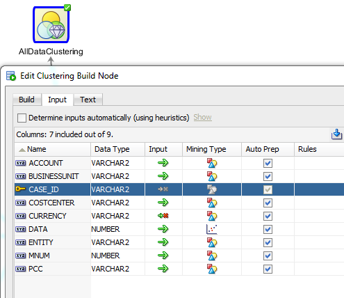
Below are the input columns. We changed the automatic inputs to allow MNUM (month number) to be a categorical input, and not data.

Once the node finished running let's review the results. For each of the algorithms we get a tree that depicts the clusters:

K-Mean (a partial diagram - it actually ends up with 19 clusters, 10 of which are leaves):

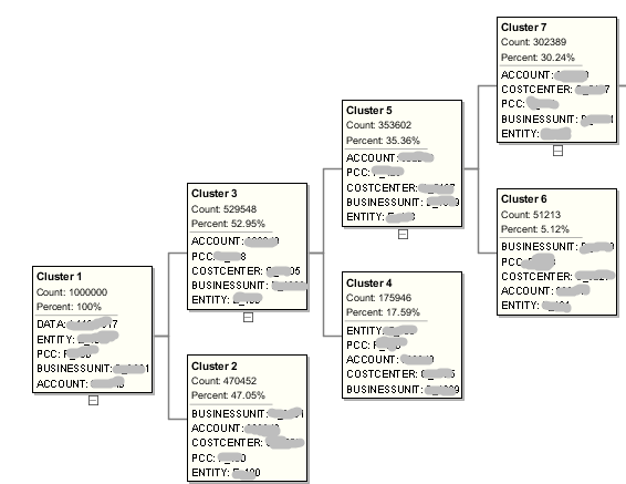
Each leaf cluster is essentially a subcube, but members from each dimension do not need to be continuous level-0 members. It’s like a multidimensional jigsaw puzzle, when each piece does not overlap with other pieces.
Each cluster has a rule such as:

If BUSINESSUNIT In ("B_xxxx") And COSTCENTER In ("C_0001", "C_0034", "C_0932", ...) And ACCOUNT In ("675675", "345565", "345346", "xxxxx",...) And PCC In ("P_xxx", "P_xxy", "P_fgh",...) And ENTITY In ("E_657", "E_345", "E_xxx", ...) Then Cluster is: 12

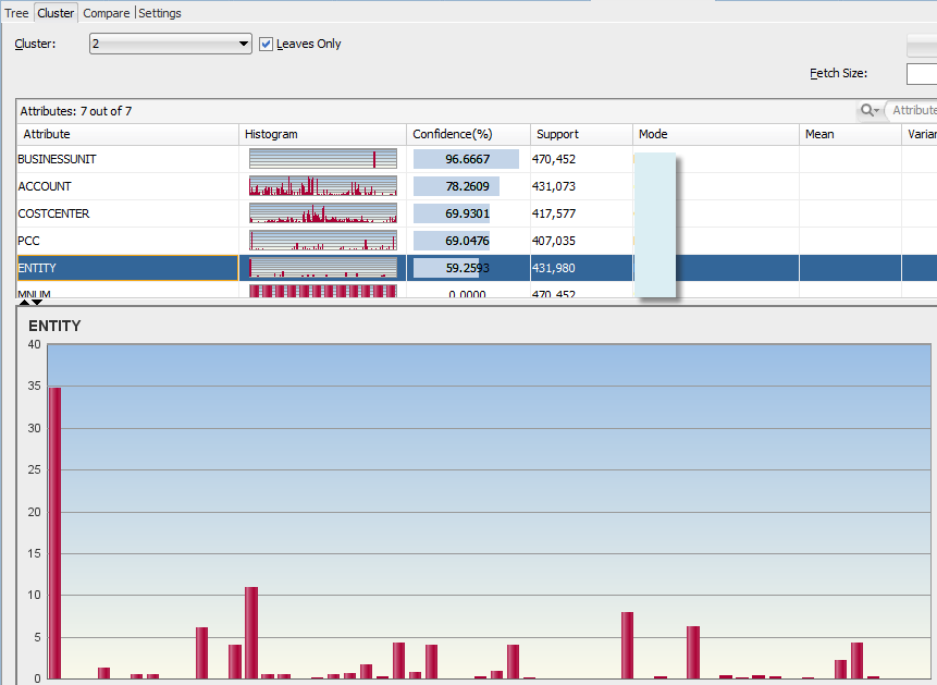
You can also see the histograms of members within each cluster:

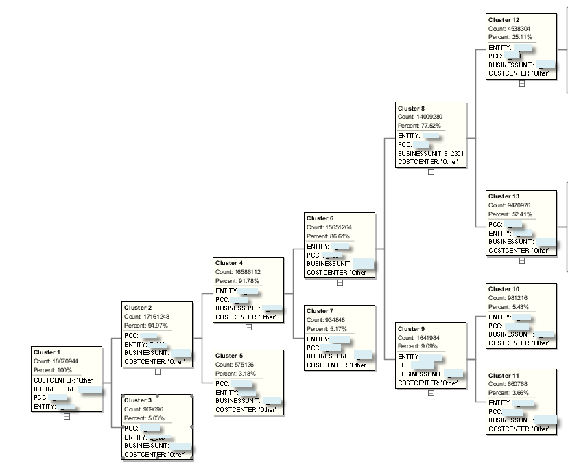
Clusters created by different algorithms are not the same. For example Expectation Maximization tree would look like this:

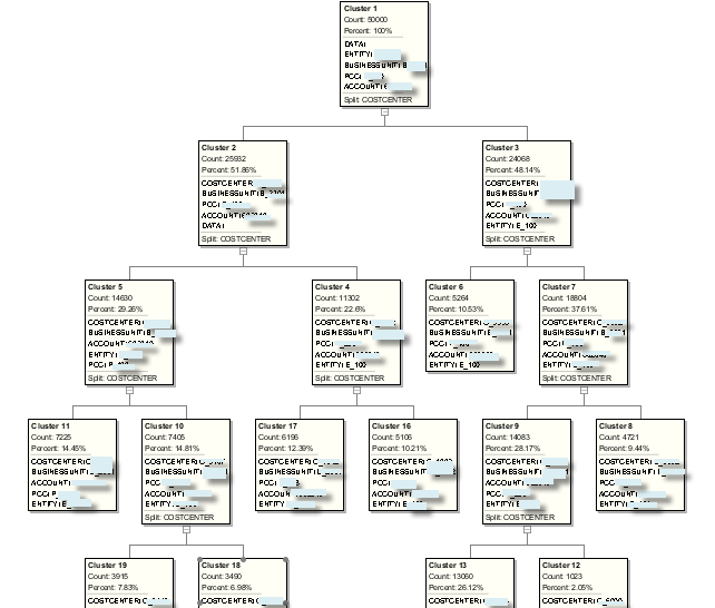
And O-cluster algorithm will generate the following tree:

So which clustering method should we use, and are their better/alternative algorithms that are not available in ODM? Different methods use different optimization techniques. For example the idea behind K-means clustering is that a good clustering is one for which the within-cluster variation is as small as possible. - Gareth James, Daniela Witten, Trevor Hastie Robert Tibshirani, “An Introduction to Statistical Learning with Applications in R”. Expectation maximization uses iterative method for finding maximum likelihood estimates of parameters. The theory behind that is beyond the scope of this post, so at this point let's assume we'll choose the algorithm based on the accuracy it produces, when we run prediction models for each cluster. 

Now, let’s recall that we run a clustering algorithm on the raw fact data that contains only level-0 members. Would it make sense to consider hierarchies? Hierarchies and different levels in them are already a form of grouping (clustering) of members by some business criteria. So if we can incorporate that “hierarchical pre-clustering” in our clustering algorithm, we would at least save time running clustering models. What about cluster accuracy? Let's review the following example.

To incorporate hierarchical information we would need to run clustering on a query that joins fact table with dimension view and returns ancestor members from different dimension levels. This is similar to how we analyzed histograms with different generations of cost center dimension.

Let’s add 2nd and the 3rd generations  of Cost Center dimension to clustering node. If we compare confidence % of K-means clusters we can see that usually the higher we go up the hierarchy the lower is the confidence. Horizontal axis represents level-0 clusters.

This makes sense once you consider what confidence % means: “Confidence is the probability that a case described by this rule will actually be assigned to the cluster.” Assume the rule for COSTCENTER in cluster 6 is {IF “C_001”, “C_002”, “C_003” THEN CLUSTER6} and it has confidence of 100%. Meaning if an observation is in either of those cost centers then it is definitely in cluster 6. Assume also that all 3 cost centers belong to a common parent VP_010,  but VP_010 also has a child C_004. What is the confidence of the rule {IF "VP_010" THEN CLUSTER6}? If an observation has attribute VP_010 it may not belong to CLUSTER6, since there is a positive probability that the level-0 Cost Center of that observation is C_004. That's why the confidence decreases when we go up the hierarchy.

So can we say that using level-0 members will always bring better results than using higher level parents? Before we answer this let's recognize the following:

• Clustering methods utilize heuristic algorithms to converge to local optimums.
• In case of K-means we predefine the number of clusters, which is 10 by default.
• Clustering algorithms are computationally expensive.

So how can we be sure that 10 clusters will really generate the best accuracy of our forecast in the end? Or is it more like 100 clusters? Or 347? The bottom line we’ll need to experiment and compare the results. But since each iteration of clustering may take quite some time, we may want to go up the hierarchy knowing that it will reduce the confidence, but will allow us to include more iterations and run the algorithm for larger number clusters, given the same time constraint.

For now let’s just keep in mind that we’ll need to run multiple iterations of clustering that will give us sub-optimal number of clusters and generation numbers for each hierarchy. Obviously this will require a lot of automation and PL/SQL code. Trying to do this in Data Miner UI seems to be non-practical. I’ll cover automation in one of the following posts.