
Automatically Generated Focused Aggregations for
Essbase
Dmitry Kryuk <hookmax@gmail.com>
Creation Date: May 20, 2015
Last updated: May 20, 2015
Version: 1.0
Abstract
On The Efficiency
One Dimension in Rows: Focused Agg Efficiency
One Dimension in Rows: Native Agg Efficiency
Multiple Dimension in Rows: Focused Agg Efficiency
Aggregations Based on Transaction Log
Calculating for every cell (bad idea)
Calculating for shared ancestors
Do we need to reinvent the wheel (@ILANCESTORS)?
Compare to the native AGG
Reinventing The Wheel
Members Classification
Constructing the Aggregation
Performance Stats
Abstract
In this series of posts we will consider different options to automate generation of focused aggregations for Essbase and Hyperion Planning.
It is well known that Hyperion Planning provides ability to design focused aggregations and run them on save. This creates real-time view of aggregated data. It also solves many issues related to scheduled calculations, like long maintenance windows, and the need to wait hours until the next calculation to see updated aggregated data.
But in reality the transition from scheduled calculations to focused business rules usually has many roadblocks. You need to use Smartview, Planning, and redesign your calculations. Most importantly, you need to change your business processes. What if organization is already using essbase extensively, and has thousands of excel templates? Now you need to convince users to switch from excel add-in to Smartview, convert their templates to predefined planning forms, and limit their ability to report and submit data. This can be an uphill battle with many casualties and tiny chances to win.
lets imagine for a moment that you are lucky enough to be on a new project which implements Planning and you design your focused Business Rules by the book.
It is trivial to develop focused aggregations for 3 or 4 dimensions, but aggregations become more complex for larger number of dimensions. True, it is the same algorithm regardless of the number of dimensions. But, if you write your focused calculation for say 6 dimensions (although it is usually unrealistic number), the script itself becomes large, and you can make an error going through all aggregation combinations, especially when you have multiple dimensions in rows/columns.
Workarounds like using user variables for rows/columns, require additional maintenance, development effort, and from the user - defining those variables.
Another aspect is testing. Considering the fact that requirements and forms layout change multiple times throughout life cycle of a standard project, focused aggregations redesign and testing could consume significant portion of the budget.
Also, are focused Business Rules really give us best possible performance? Can we optimize aggregations even more? When we have one or more dimensions in the rows, it is unlikely that all rows are being changed every time the form is submitted. Sometimes forms have hundreds or thousands of rows simply because they inherited their design from Excel Add-in templates. If only 1% of rows has actually changed, and if we aggregate for 100% of the rows, the aggregation is not really a focused or efficient, is it?
So we have 3 issues on our hands:
- Users are not willing to use Planning forms or to switch from excel add-in to Smartview
- Implementation budget for planning, and focused BRs is much higher (due to development costs, but also because of licensing fees and infrastructure footprint)
- Even if we do implement focused BRs, they do not guarantee optimal performance, if users keep the structure of the old excel templates.
So, can we run efficient focused calculations, let users work the way they are used to, and do this for a fraction of the budget considering the alternatives? This is what we try to explore in this post. And first we need to dive into technical stuff. If, however, you want to go directly to the description of the method that constructs focused aggregations automatically, you can jump to Reinventing The Wheel section.
On The Efficiency
One Dimension in Rows: Focused Agg Efficiency
An example of suboptimal approach to focused aggregation is a use of a variable to specify a member, descendents of which are displayed in the form. Then descendents and ancestors of that member are aggregated in calculation.
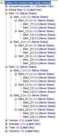
Lets consider the outline below, and use a member Dim1_11 as a value for user variable.
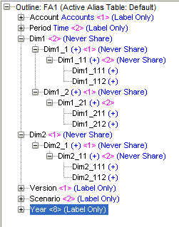
Descendents of Dim1_11, members Dim1_111 and Dim1_112 are displayed in the form as rows. For simplicity assume Dim2 has a similar hierarchy structure, and its level 0 members are displayed in a page drop-down. Member Dim2_112 is selected. Something like the form below:
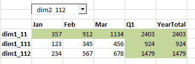
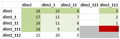
Also assume we have data in 4 level 0 combinations, and we already aggregated the data once. Now we updated Dim1_111->Dim2_112 combination.
The matrix below shows the updated cell, and numbers show the order of calculation.
The following calculation would be used to aggregate a webform. Obviously, specific member names would be substituted with run-time-prompts and variables.
/*---Script BR001---*/
SET MSG DETAIL;
SET UPDATECALC OFF;
SET CLEARUPDATESTATUS OFF;
SET EMPTYMEMBERSETS ON;
SET CACHE DEFAULT;
/*-----Part1---------*/
FIX("DIM2_112")
@IDESCENDANTS("DIM1_11");
@ANCESTORS("DIM1_11");
ENDFIX
/*-----Part2---------*/
FIX(@IDESCENDANTS("DIM1_11"), @ANCESTORS("DIM1_11"))
@ANCESTORS("DIM2_112");
ENDFIX
|
If only one member was updated on the form (say Dim1_111), we would need to calculate only 15 cells that were impacted by the change:
(3 ancestors of dim1_111 + dim1_111 member itself)x(3 ancestors of dim2_112 + dim2_112 member itself) - changed level-0 combination.
What happened in practice? Below is the output from the calculation.
The output from the first FIX:
Output from Script BR001 - Part1
Calculating [ Dim1(Dim1_111,Dim1_112,Dim1_11,Dim1_1,Dim1)] with fixed members [Dim2(Dim2_112)].
Executing Block - [Dim1_11], [Dim2_112], [Working], [BUDGET], [FY14].
Executing Block - [Dim1_1], [Dim2_112], [Working], [BUDGET], [FY14].
Executing Block - [Dim1], [Dim2_112], [Working], [BUDGET], [FY14].
Total Block Created: [0.0000e+00] Blocks
Sparse Calculations: [3.0000e+00] Writes and [8.0000e+00] Reads
Dense Calculations: [0.0000e+00] Writes and [0.0000e+00] Reads
Sparse Calculations: [3.9000e+01] Cells
Dense Calculations: [0.0000e+00] Cells.
|
One thing to notice is the number of reads. While executing the block, Essbase reads all child blocks and currently calculated block. So to calculate
Dim1_11 Essbase reads blocks Dim1_111, Dim1_112 and Dim1_11 itself.
Dim1_1: reads blocks Dim1_11, Dim1_1
Dim1: reads blocks Dim1_11, Dim1_12, Dim1.
Hence, we have the total of 8 blocks to read appearing in the output.
The output from the second FIX:
Output from Script BR001 - Part2
Calculating [ Dim2(Dim2_11,Dim2_1,Dim2)] with fixed members [Dim1(Dim1_111, Dim1_112, Dim1_11, Dim1_1, Dim1)].
Executing Block - [Dim1_111], [Dim2_11], [Working], [BUDGET], [FY14].
Executing Block - [Dim1_11], [Dim2_11], [Working], [BUDGET], [FY14].
Executing Block - [Dim1_1], [Dim2_11], [Working], [BUDGET], [FY14].
Executing Block - [Dim1], [Dim2_11], [Working], [BUDGET], [FY14].
Executing Block - [Dim1_111], [Dim2_1], [Working], [BUDGET], [FY14].
Executing Block - [Dim1_11], [Dim2_1], [Working], [BUDGET], [FY14].
Executing Block - [Dim1_1], [Dim2_1], [Working], [BUDGET], [FY14].
Executing Block - [Dim1], [Dim2_1], [Working], [BUDGET], [FY14].
Executing Block - [Dim1_111], [Dim2], [Working], [BUDGET], [FY14].
Executing Block - [Dim1_11], [Dim2], [Working], [BUDGET], [FY14].
Executing Block - [Dim1_1], [Dim2], [Working], [BUDGET], [FY14].
Executing Block - [Dim1], [Dim2], [Working], [BUDGET], [FY14].
Total Block Created: [0.0000e+00] Blocks
Sparse Calculations: [1.5000e+01] Writes and [3.5000e+01] Reads
Dense Calculations: [0.0000e+00] Writes and [0.0000e+00] Reads
Sparse Calculations: [1.5600e+02] Cells
Dense Calculations: [0.0000e+00] Cells.
|
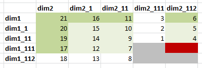
Total Block Created = 0 since the database was preaggregated. The changed cell had value already before it was changed.
But instead of 15 blocks we calculated 18 blocks. This is because we have 2 rows on a form, and our calculation is designed to calculate all rows. Hence the efficiency of our calculation is 83% . the metric for efficiency would simply be the optimal number of blocks that need calculation divided by the actual calculated number. So The best efficiency is 100%, and the worse it becomes it asymptotically converge to 0.
It may seem like not a big deal - losing 17% of efficiency, but we’ll see later that lost efficiency grows fast.
The generic formula for the lower limit of the number of cells to be calculated:
Cmin=d=1D(kd+|jkdA(mjd)|)-d=1D(kd)
Whereas:
kd is number of updated level-0 members of d-th dimension
mjdis the updated j-th member of d-th dimension
|A(mjd)| - the number of all ancestors of mjd
jkdA(mjd) - union of all ancestor sets of members mjd
In our example:
mj1=d1-111 , mj2=d2-112
jk1A(mj1)=A(m11)={d1-11,d1-1,d1}
jk2A(mj2)=A(m12)={d2-11,d2-1,d2}
|jk1A(mj1)|=|jk2A(mj2)|=3
k1=k2=1
Cmin= 15
One Dimension in Rows: Native Agg Efficiency
lets compare BR001 result to the calc script that uses native AGG function:
/*---Script BR001b---*/
SET MSG DETAIL;
SET UPDATECALC OFF;
SET CLEARUPDATESTATUS OFF;
SET EMPTYMEMBERSETS ON;
SET CACHE DEFAULT;
Agg("Dim1", "Dim2");
|
And the output:
Output from Script BR001b
Multiple bitmap mode calculator cache memory usage has a limit of [16666] bitmaps..
Aggregating [ Dim1(All members) Dim2(All members)].
Executing Block - [Dim1_11], [Dim2_111], [Working], [BUDGET], [FY14].
Executing Block - [Dim1_1], [Dim2_111], [Working], [BUDGET], [FY14].
Executing Block - [Dim1], [Dim2_111], [Working], [BUDGET], [FY14].
Executing Block - [Dim1_11], [Dim2_112], [Working], [BUDGET], [FY14].
Executing Block - [Dim1_1], [Dim2_112], [Working], [BUDGET], [FY14].
Executing Block - [Dim1], [Dim2_112], [Working], [BUDGET], [FY14].
Executing Block - [Dim1_111], [Dim2_11], [Working], [BUDGET], [FY14].
Executing Block - [Dim1_112], [Dim2_11], [Working], [BUDGET], [FY14].
Executing Block - [Dim1_11], [Dim2_11], [Working], [BUDGET], [FY14].
Executing Block - [Dim1_1], [Dim2_11], [Working], [BUDGET], [FY14].
Executing Block - [Dim1], [Dim2_11], [Working], [BUDGET], [FY14].
Executing Block - [Dim1_111], [Dim2_1], [Working], [BUDGET], [FY14].
Executing Block - [Dim1_112], [Dim2_1], [Working], [BUDGET], [FY14].
Executing Block - [Dim1_11], [Dim2_1], [Working], [BUDGET], [FY14].
Executing Block - [Dim1_1], [Dim2_1], [Working], [BUDGET], [FY14].
Executing Block - [Dim1], [Dim2_1], [Working], [BUDGET], [FY14].
Executing Block - [Dim1_111], [Dim2], [Working], [BUDGET], [FY14].
Executing Block - [Dim1_112], [Dim2], [Working], [BUDGET], [FY14].
Executing Block - [Dim1_11], [Dim2], [Working], [BUDGET], [FY14].
Executing Block - [Dim1_1], [Dim2], [Working], [BUDGET], [FY14].
Executing Block - [Dim1], [Dim2], [Working], [BUDGET], [FY14].
Total Block Created: [0.0000e+00] Blocks
Sparse Calculations: [2.1000e+01] Writes and [4.9000e+01] Reads
Dense Calculations: [0.0000e+00] Writes and [0.0000e+00] Reads
Sparse Calculations: [2.7300e+02] Cells
Dense Calculations: [0.0000e+00] Cells.
|
Nothing is terribly surprising. Complete aggregation across two dimensions has written and read more blocks than the focused aggregation. Now consider this fact: Our database contained data in 4 level 0 cells (marked in grey). So by running focused aggregation we calculated 50% of the existing data set. And when we used native AGG we calculated complete data set.
What happens if we clear the database and input data into a single cell, the one that is a focus of our focused aggregation (dim1_111-->dim2_112)? Lets rerun both BR001 and BR001b calculations.
Read/Writes for BR001:
Sparse Calculations: [3.0000e+00] Writes and [8.0000e+00] Reads
Sparse Calculations: [1.2000e+01] Writes and [2.8000e+01] Reads
Read/Writes for BR001b:
Sparse Calculations: [1.5000e+01] Writes and [3.0000e+01] Reads
The order of calculated cells is identical for both:
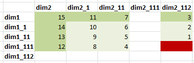
Figure 4.
Well, in this case complete agg is more efficient than focused agg, since it had to read only 30 blocks instead of 36. But we are not comparing apples to apples here, and the reason is this line in the log:
Calculator Cache With Multiple Bitmaps For: [Currency].
|
In our focused aggregation we notice this in the output:
Calculator Cache: [Disabled].
|
Why was calculator cache disabled for focused aggregation? Because by default it is enabled only when at least one full sparse dimension is calculated. To override that default we used SET CACHE ALL; statement. To have consistent results we either need to SET CACHE ALL for focused calculations, or SET CACHE OFF for native AGG. If we disable calc cache for native AGG we get the same
Sparse Calculations: [1.5000e+01] Writes and [3.6000e+01] Reads
|
In further examples we disable calculator cache for consistency.
Multiple Dimension in Rows: Focused Agg Efficiency
What happens if we put 2 dimensions in the rows? Lets say we have 4 combinations of level 0 members in rows:
If only one combination gets updated, say Dim1_111->Dim2_112 we would still need to calculate only 15 cells. Although layout of the form has changed, nothing changed from calculation requirements perspective. Those are the same cells from the previous example.
But since our aggregation needs to take care of 2 dimensions brought into rows, our script is based on descendant and ancestors of Dim1_11 and Dim2_11. This is how it looks like:
/*---Script BR002---*/
FIX(@RELATIVE("DIM2_11",0))
@IDESCENDANTS("DIM1_11");
@ANCESTORS("DIM1_11");
ENDFIX
FIX(@IDESCENDANTS("DIM1_11"), @ANCESTORS("DIM1_11"))
@IDESCENDANTS("DIM2_11");
@ANCESTORS("DIM2_11");
ENDFIX
|
And this is the output:
Output from Script BR002
Calculating [ Dim1(Dim1_111,Dim1_112,Dim1_11,Dim1_1,Dim1)] with fixed members [Dim2(Dim2_111, Dim2_112)].
Executing Block - [Dim1_11], [Dim2_111], [Working], [BUDGET], [FY14].
Executing Block - [Dim1_1], [Dim2_111], [Working], [BUDGET], [FY14].
Executing Block - [Dim1], [Dim2_111], [Working], [BUDGET], [FY14].
Executing Block - [Dim1_11], [Dim2_112], [Working], [BUDGET], [FY14].
Executing Block - [Dim1_1], [Dim2_112], [Working], [BUDGET], [FY14].
Executing Block - [Dim1], [Dim2_112], [Working], [BUDGET], [FY14].
Sparse Calculations: [6.0000e+00] Writes and [1.6000e+01] Reads
Calculating [ Dim2(Dim2_111,Dim2_112,Dim2_11,Dim2_1,Dim2)] with fixed members [Dim1(Dim1_111, Dim1_112, Dim1_11, Dim1_1, Dim1)].
Executing Block - [Dim1_111], [Dim2_11], [Working], [BUDGET], [FY14].
Executing Block - [Dim1_112], [Dim2_11], [Working], [BUDGET], [FY14].
Executing Block - [Dim1_11], [Dim2_11], [Working], [BUDGET], [FY14].
Executing Block - [Dim1_1], [Dim2_11], [Working], [BUDGET], [FY14].
Executing Block - [Dim1], [Dim2_11], [Working], [BUDGET], [FY14].
Executing Block - [Dim1_111], [Dim2_1], [Working], [BUDGET], [FY14].
Executing Block - [Dim1_112], [Dim2_1], [Working], [BUDGET], [FY14].
Executing Block - [Dim1_11], [Dim2_1], [Working], [BUDGET], [FY14].
Executing Block - [Dim1_1], [Dim2_1], [Working], [BUDGET], [FY14].
Executing Block - [Dim1], [Dim2_1], [Working], [BUDGET], [FY14].
Executing Block - [Dim1_111], [Dim2], [Working], [BUDGET], [FY14].
Executing Block - [Dim1_112], [Dim2], [Working], [BUDGET], [FY14].
Executing Block - [Dim1_11], [Dim2], [Working], [BUDGET], [FY14].
Executing Block - [Dim1_1], [Dim2], [Working], [BUDGET], [FY14].
Executing Block - [Dim1], [Dim2], [Working], [BUDGET], [FY14].
Sparse Calculations: [1.5000e+01] Writes and [3.5000e+01] Reads
|
Now we aggregate 21 cells including level 0 blocks. Hence our efficiency degrades to 71%. This is exactly the same result as in the case when we used native Agg across 2 dimensions. And not surprisingly, since we do aggregate 2 dimensions entirely. Since both dimensions are in the row we cannot benefit from focused aggregation.
To summarize we saw the following factors affecting the efficiency of focused aggregations:
- The number of rows/columns updated by the user: the lower the percentage of rows/columns being updated, the higher percentage of blocks being needlessly aggregated. Hence the lower efficiency. We saw this in the first example.
- The number of dimensions we put in rows/columns. The more dimensions we put - the less efficient focused aggregation becomes. We saw this in the example of multiple dimensions in the rows.
- The larger percent of the existing data is being updated, the more efficient native agg becomes.
Aggregations Based on Transaction Log
In previous section the assumption was that focused aggregations are driven by web form layout. Lets assume now we don’t need any front-end application, that will define the structure of our focused calculation. Instead, lets assume the users continues to use their excel add-in, and there are no planning forms. But we enabled transactions logging and are going to generate focused aggregations based on transactions.
Calculating for every cell (bad idea)
Assume we can identify the specific cell that has changed. To create a focused aggregation for that cell in a one-dimensional database, we would simply calculate all ancestors of a given member. Then we would get to the next cell, and would repeat… But wait, those cells may have some common ancestors. In the best case only 1 ancestor - top dimension node. In the worst case - if 2 members are siblings, all ancestors will be the same, and we would redundantly calculate them.
Consider also that changed level-0 cells usually come in batches with similar dimensionality - either from Planning forms, Smartview, or other sources. And if the batch contains 1000 cells, running individual focused calculation for each one will result in super-inefficient overall performance due to redundant calculations of upper levels.
To illustrate this point let us modify our data entry and see how it works. Below is the slightly modified outline:
and data form:
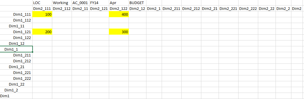
How does the calculation order look like if we just run focused aggregation for every changed cell by using @Ancestors function?
/*---Script BR004b---*/
//ESS_LOCALE English_UnitedStates.Latin1@Binary
/*---Script BR001---*/
SET MSG DETAIL;
SET UPDATECALC OFF;
SET CLEARUPDATESTATUS OFF;
SET EMPTYMEMBERSETS ON;
SET CACHE DEFAULT;
FIX("Working","BUDGET","LOC","FY14")
/*-----Part1---------*/
FIX("Dim2_111","Dim2_122")
@ANCESTORS("DIM1_111");
@ANCESTORS("DIM1_121");
ENDFIX
/*-----Part2---------*/
FIX(@IANCESTORS("DIM1_111"),@IANCESTORS("DIM1_121"))
@ANCESTORS("Dim2_111");
@ANCESTORS("Dim2_122");
ENDFIX
ENDFIX
|
Now we have expected results:
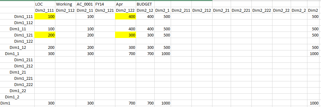
But undesirable cells order:
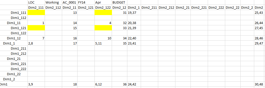
Some cells have 2 order numbers, meaning they are calculated twice.
16 cells are calculated twice out of lowest possible 32. Hence our efficiency is only 32/48=66%.
The output:
Total Block Created: [8.0000e+00] Blocks
Sparse Calculations: [1.2000e+01] Writes and [3.6000e+01] Reads
Total Block Created: [2.4000e+01] Blocks
Sparse Calculations: [3.6000e+01] Writes and [1.0800e+02] Reads
|
So what’s the problem - you ask. Just remove redundancy by composing focused aggregation for the complete batch (changed set)!
Ok, this is indeed what we are going to try.
Calculating for shared ancestors
The idea is to construct a list of ancestors, similar to @IALLANCESTORS function, but for a set instead of for a single member. In the diagram below changed level-0 cells are represented by red circles. Green pluses represent their ancestors that need calculation.
But wait a seconds, isn’t there a function @ILANCESTORS that does exactly that? From technical reference:
@ILANCESTORS
Returns the members of the specified member list and either all ancestors of the members or all ancestors up to the specified generation or level.
You can use the @ILANCESTORS function as a parameter of another function, where the function requires a list of members. The result does not contain duplicate members.
Example
@ILANCESTORS(@LIST(“100–10”,"200–20”))
Do we need to reinvent the wheel (@ILANCESTORS)?
The following script:
/*---Script BR004a---*/
SET MSG DETAIL;
SET UPDATECALC OFF;
SET CLEARUPDATESTATUS OFF;
SET EMPTYMEMBERSETS ON;
SET CACHE DEFAULT;
FIX("Working","BUDGET","LOC","FY14")
/*-----Part1---------*/
FIX("Dim2_111","Dim2_122")
@ILANCESTORS(@LIST("DIM1_111","Dim1_121"));
ENDFIX
/*-----Part2---------*/
FIX(@ILANCESTORS(@LIST("DIM1_111","Dim1_121")))
@ILANCESTORS(@LIST("Dim2_111","Dim2_122"));
ENDFIX
ENDFIX
|
And results:
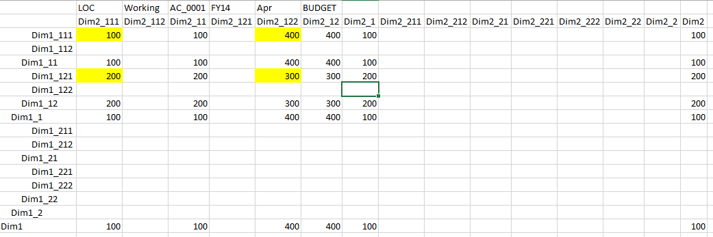
Hmm… not exactly what we expected. And the reason is evident from the blocks execution order. Numbers below show the order of execution:
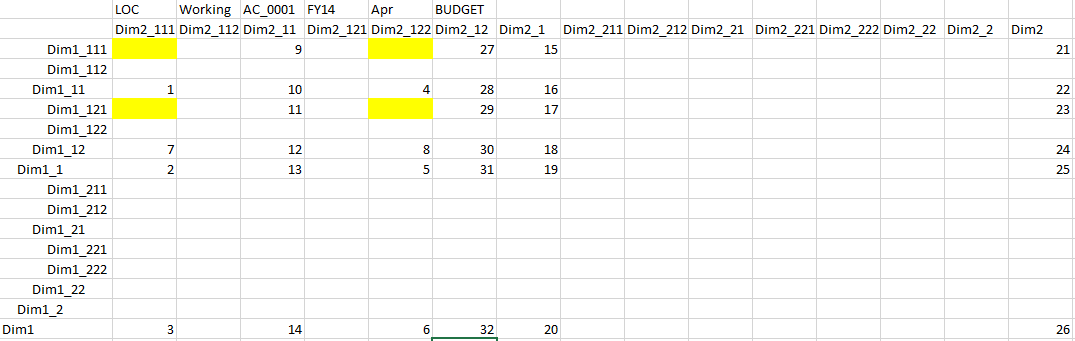
You can see from the order of execution that @ILANCESTORS function generates ancestors for the first member in the list (Dim1_11, Dim1_1, Dim1), and then ancestors for the second member (Dim1_12, Dim1_1, Dim1). But remember the statement from the tech ref: “The result does not contain duplicate members”? that’s why Dim1_1, Dim1 are removed from the set of ancestors of the second member. So we end up with Dim1_11, Dim1_1, Dim1, Dim1_12. Which is clearly not what we want. The second calculation part of Dim2 works the same way: calculation order is Dim2_11,Dim2_1,Dim2, Dim2_12.
The peculiar fact is that the order of @ILANCESTORS generated ancestors in the FIX is different: Dim1_111, Dim1_11, Dim1_121, Dim1_12, Dim1_1, Dim1.
But in terms of the efficiency we have written 32 blocks and read 96 blocks, so we get 100% efficiency (if we take into consideration only writes). Here’s the output:
Total Block Created: [8.0000e+00] Blocks
Sparse Calculations: [8.0000e+00] Writes and [2.4000e+01] Reads
Total Block Created: [2.4000e+01] Blocks
Sparse Calculations: [2.4000e+01] Writes and [7.2000e+01] Reads
|
Compare to the native AGG
Just for the record, lets see how it looks if we use a regular Agg. Since 4 changed cells is all we have in the database we would expect 100% efficiency from native AGG as well.
/*---Script BR004c---*/
//ESS_LOCALE English_UnitedStates.Latin1@Binary
/*---Script BR001---*/
SET MSG DETAIL;
SET UPDATECALC OFF;
SET CLEARUPDATESTATUS OFF;
SET EMPTYMEMBERSETS ON;
SET CACHE DEFAULT;
FIX("Working","BUDGET","LOC","FY14")
Agg("Dim1","Dim2");
ENDFIX
|
Results are obviously as expected, as well as the read/write results:
Total Block Created: [3.2000e+01] Blocks
Sparse Calculations: [3.2000e+01] Writes and [9.6000e+01] Reads
Dense Calculations: [0.0000e+00] Writes and [0.0000e+00] Reads
|
These are exactly the same numbers when we used @ILANCESTORS function.
Reinventing The Wheel
We saw that we cannot use @ILAncestors function, but in terms of efficiency it is as efficient as it gets. So how about we create our own function that would return sets of ancestors properly ordered?
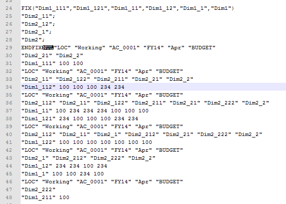
To accomplish this we will use essbase Java API and will parse the transactions log. When you enable transactions logging essbase registers all changes to the data. So even if a user has a huge excel-add-in template with 600,000 cells, out of which only a few hundreds had changed, transaction log will write only changed cells.
In the screenshot below you can see that the log contains calculation script and then data submitted from Smartview ad-hoc analysis.
Members Classification
From this chunk of log we need to get 2 things:
- Dimensions and members that need to be aggregated, and used in construction of focused aggregation.
- Dimensions that do not need to be aggregated, and are used in POV section of the calc script.
This information does not show up in the log. But we can distinguish a data point from a member name.
And we can see where one transaction starts and where it ends.
The rest we can do by connecting to essbase database, and getting additional information about each member.
We can find out:
- To which dimension the member belongs
- Who is its parent
- Get its ancestors up to the top node
- Get generation of each parent
- Their storage type.
This is enough to
- Categorize members that show up in transactions by dimensions
- Get distinct set of their ancestors
- Order them by generation
- Based on storage property of each ancestor, classify whether dimension is as POV or it should participate in focused aggregation.
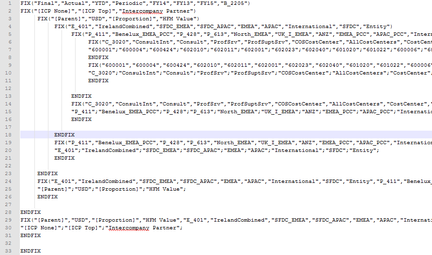
Below are results of member/dimension classification:
Version: {Final=-2.0}
Scenario: {Actual=-2.0}
Version: {Final=-2.0}
Scenario: {Actual=-2.0}
View: {YTD=-2.0, Periodic=-2.0}
Year: {FY14=-2.0, FY13=-2.0, FY15=-2.0}
Intercompany Partner: {[ICP None]=-3.0, [ICP Top]=-2.0, Intercompany Partner=-1.0}
HFM Value: {[Parent]=-3.0, USD=-3.0, [Proportion]=-2.0, HFM Value=-1.0}
Entity: {E_401=-7.0, IrelandCombined=-6.0, SFDC_EMEA=-5.0, SFDC_APAC=-5.0, EMEA=-4.0, APAC=-4.0, International=-3.0, SFDC=-2.0, Entity=-1.0}
PCC: {P_411=-8.0, Benelux_EMEA_PCC=-7.0, P_428=-7.0, P_613=-7.0, North_EMEA=-6.0, UK_I_EMEA=-6.0, ANZ=-6.0, EMEA_PCC=-5.0, APAC_PCC=-5.0, International_PCC=-4.0, SFDC_PCC=-3.0, AllPCCs=-2.0, PCC=-1.0}
BusinessUnit: {B_2205=-7.0}
CostCenter: {C_3020=-8.0, ConsultInt=-7.0, Consult=-6.0, ProfSrv=-5.0, ProfSuptSrv=-4.0, COSCostCenter=-3.0, AllCostCenters=-2.0, CostCenter=-1.0}
Account: {600001=-12.0, 600004=-12.0, 600424=-12.0, 602010=-12.0, 602011=-12.0, 602001=-12.0, 602023=-12.0, 602040=-12.0, 601020=-12.0, 601022=-12.0, 600006=-12.0, 600426=-12.0, 601021=-12.0, 601024=-12.0, 600420=-12.0, 601000=-12.0, 600430=-11.0, 600440=-11.0, 603000=-11.0, 642000=-11.0, 642003=-11.0, 642004=-11.0, 650001=-10.0, 650002=-10.0, 650005=-10.0, 650006=-10.0, 651000=-10.0, 651002=-10.0, ConsFuncNonGAAP=-10.0, ConsFunc=-10.0, 641001=-10.0, 650000=-10.0, 650003=-10.0, 650004=-10.0, 832001=-10.0, 640001=-10.0, 810001=-9.0, 960106=-9.0, 811000=-9.0, 830002=-9.0, 812000=-9.0, 812003=-9.0, 820000=-8.0, 820002=-8.0, 910002=-7.0, 910007=-7.0, 910008=-7.0, 690000=-6.0, 690020=-6.0, PERFTE=-5.0, MRATE=-5.0, ValidateNonGAAP=-4.0, ACCRUALRATES=-4.0}
dimProperties: {Version=, Scenario=, View=, Year=, Intercompany Partner=Has Parents: Intercompany Partner;, HFM Value=Has Parents: HFM Value;, Entity=Has Parents: Entity;, PCC=Has Parents: PCC;, BusinessUnit=, CostCenter=Has Parents: CostCenter;, Account=Has Parents: ACCRUALRATES;}
================================
AGGREGATED DIMENSIONS: {1=Intercompany Partner, 2=HFM Value, 3=Entity, 4=PCC, 5=CostCenter, 6=Account}
POV: {1=Version, 2=Scenario, 3=View, 4=Year, 5=BusinessUnit}
|
These results are based on a different database with real data volume and with large transactions going through ad-hoc reporting.
You see that there are 6 dimensions that require aggregation. The rest are POV dimensions. All ancestors of the members from POV dimensions are dynamic calc or label only members. Lets take a look at one of the aggregated dimensions, PCC for example. Members are ordered by generation. On the other hand dimension like Year has a single generation =2, meaning it does not need to be aggregated.
While parsing members we should also take into consideration shared members, but we will not get into that here.
Constructing the Aggregation
Once we have members classifications, we can start constructing the calculation. But how can that be done automatically? The algorithm is pretty simple. You just need to generate focused aggregation for 3 dimensions and then extend it to any number of dimensions.
Lets write a pseudocode for 3 dimensions. @GETCHANGEDSET is a function that returns all changed members of one dimension ordered properly.
FIX (@GETCHANGEDSET(Dim1))
FIX (@GETCHANGEDSET(Dim2))
@GETCHANGEDSET(Dim3);
ENDFIX
FIX (@GETCHANGEDSET(Dim3))
@GETCHANGEDSET(Dim2);
ENDFIX
ENDFIX
FIX (@GETCHANGEDSET(Dim2))
FIX (@GETCHANGEDSET(Dim3))
@GETCHANGEDSET(Dim1);
ENDFIX
ENDFIX
|
You can see that we put each dimension forward for aggregation, while the rest become fixed dimensions.
FIX FIX AGG
Dim1 Dim2 Dim3
Dim1 Dim3 Dim2
Dim3 Dim2 Dim1
For 4 dimensions aggregation plan would look like this.
FIX FIX FIX AGG
Dim1 Dim2 Dim3 Dim4
Dim1 Dim2 Dim4 Dim3
Dim1 Dim4 Dim3 Dim2
Dim4 Dim3 Dim2 Dim1
And for N dimensions:
FIX FIX FIX AGG
Dim1 Dim2 ... DimN
Dim1 Dim2 ... DimN-1
Dim1 Dim2 ... DimN-2
… … … ...
DimN DimN-1 ... Dim1
Now lets transform the code into recursive form. {REDUCED FORM FOR 2 DIMENSIONS} is the reduction of our problem from 3 dimensions to 2 dimensions.
FIX (@GETCHANGEDSET(Dim1))
{REDUCED FORM FOR 2 DIMENSIONS}
ENDFIX
FIX (@GETCHANGEDSET(Dim2),@GETCHANGEDSET(Dim3)
@GETCHANGEDSET(Dim1);
ENDFIX
|
Once we reduced the problem we can solve it for any number of dimensions. So for N dimensions it would look like this:
FIX (@GETCHANGEDSET(Dim1))
{REDUCED FORM FOR N-1 DIMENSIONS}
ENDFIX
FIX (@GETCHANGEDSET(DimN),@GETCHANGEDSET(N-1)...@GETCHANGEDSET(2))
@GETCHANGEDSET(Dim1);
ENDFIX
|
Lets come back to our transaction and see how focused aggregation would look like.
Notice that this calculation is:
- Generated automatically for the specific data set that has changed. So it wouldn’t matter how many dimensions we have in the rows or columns.
- Since it doesn’t contain extra members that haven’t changed in terms of writing blocks its efficiency is better than the using focused aggregations in BRs, based on RTPs provided from the form.
- If you implement this method you don’t need to write a single line of code to create focused aggregations for all existing forms, or to change them when users want to change forms.
Performance Stats
In our previous example there were 11 dimensions in the database, and transaction contained 3912 changed cells. It had 326 rows with 3586 members from all dimensions. It took 25 sec to parse and classify all members and to create focused aggregation. And it took 14 sec to execute the aggregation.
In other examples of large transactions, parsing and calculations took around 9 ms per changed cell. In more reasonable example of a template that contained 52 rows and 12 columns, calculation took 5.5 sec.
For small transaction of 1 row and 12 columns the overhead of parsing was 0.4 sec, and total time was .7 sec. Compare this to 40 min that takes complete aggregation of the database. Obviously it would also depend on the database structure and how transaction data is distributed across multiple dimensions.
Rows
|
Members
|
Cells
|
Parsing (sec)
|
Calc
(sec)
|
Total (sec)
|
Time Per Cell (ms)
|
36446
|
400950
|
437352
|
318
|
64
|
382
|
0.873438
|
326
|
3586
|
3912
|
25
|
14
|
39
|
9.969325
|
101
|
1111
|
1212
|
5
|
5
|
10
|
8.250825
|
52
|
566
|
624
|
3
|
2.5
|
5.5
|
8.814103
|
1
|
11
|
12
|
0.4
|
0.29
|
0.69
|
57.5
|
In the next post we will discuss how to optimize calculations even more considering the fact that multiple users will submit their data concurrently, so if they run calculations independently some of the calculations for upper blocks will be repeated.
We will also consider integration options: which mechanism will monitor changing transactions log, and will execute generated scripts.
No comments:
Post a Comment