Tuesday, June 30, 2015

Testing Hyperion Planning with LoadRunner and ALM Performance Center

Dmitry Kryuk <hookmax@gmail.com>

Creation Date: May 16, 2014

Last updated: May 21, 2014

Version: 1.0

Overview

Workflow

EPM Automation

Export BRs from Planning repository

Create dummy forms

Load the package with LCM

Forms Extract

Generate LoadRunner scripts based on tokenized LoadRunner blueprint.

ALM Performance Center Steps

Upload VuGen scripts

Copy test scenario blueprint.

Replace default test script in copied scenario.

Update SLAs

Update the number of virtual users.

Total number of Vusers per script.

Geographic distribution.

Copy Test Set Blueprint.

Add test from steps 7-10 to copied test set

Execute the test set.

Overview

Let’s review the workflow of performance testing with LoadRunner/ALM Performance Center.

We focus on testing of two central object types of Hyperion Planning applications: web forms and Business Rules.

We use a LoadRunner script blueprint that simulates the following actions:

Workspace authentication
Opens application
Opens webform
Saves web form

To test a business rule with this blueprint, we would have to associate BR with a web form, and define a web forms so that BR would run “On Save”, and run-time-prompts (RTPs) are not shown.

Business rules may be associated differently with the webform in tested application itself. Other usage scenarios include:

BR is triggered from “Business Rules” interface, and is not associated with any webform.
BR is associated with a web form via menus.
BR uses RTPs, but user is required to input them manually.

For those cases we need to create a dummy web form for each BR. We do not check “Use Members on Form” option since members on a dummy web form are irrelevant for a specific business rule. We rather prefer the business rule to use a default variable value. Obviously, this situation is not ideal, since data can be dispersed in such a way that a particular BR will not run on a representative data set.

Hence from the performance testing perspective we would prefer if BRs have RTPs, are associated with with real web forms, and run when the form is saved. BRs that don’t use RTPs can be tested with dummy web forms.

Workflow

EPM Automation

The diagram below describes the steps we need to perform in order to automate performance testing with third party tool like LoadRunner.

Export BRs from Planning repository

See sample SQL script in Appendix.

Create dummy forms

Create one dummy web form per application
Export the web form with LCM
Tokenize the XML file of a webform (replace values like plan type and Business Rule name with tokens). Check example of tokenized LCM form in Appendix.
Execute a script that generates XML files based on a tokenized template, and prepares LCM package to be loaded into test application. I use a python script that takes the list of BRs and a tokenized forms as parameters.

Load the package with LCM
Forms Extract

Now all our business rules are associated with a web form that will trigger the rule. Once LCM package is loaded we can extract webforms with their IDs from Planning repository. We will need those IDs in subsequent steps in order to create test scripts.

Generate LoadRunner scripts based on tokenized LoadRunner blueprint.

ALM Performance Center Steps

The diagram below describes the steps needed to prepare ALM objects for testing.

Upload VuGen scripts

We can now upload LoadRunner scripts to ALM Performance Center. Upload itself is a manual and time-consuming process. Unfortunately ALM interface does not allow bulk uploads, you have to upload 5 scripts each time.

After test script was uploaded it needs to be associated with test scenario. Test scenario includes the following information:

Test scripts to run
Load generators to use
WAN emulation configuration (Shunra)
Number of users for each test
Configuration of how the load builds up
Duration of the test
SLAs
Monitoring

Copy test scenario blueprint.

We use test scenario blueprint as a starting point. After copuing the blueprint we need to rename it. The name of a new test scenario is a web form ID being tested.

Replace default test script in copied scenario.

Test scenario copy should be modified to reflect characteristics of the tested Business Rule. The first item to update is test script names in workload interface. This needs to be updated even when an existing test script was uploaded. When ALM overwrites the existing script it deletes the old script and all objects referencing the old script become invalid. Then it uploads the new script, and creates new records in the repository. Hence all objects referencing the old script need to be updated.

Update SLAs

Existing SLAs become invalid once we updated test scripts in Workload interface. So we’ll need to delete existing and create a new SLA. In our case SLAs are defined based on 90th percentile of execution time per transaction. The following transactions are available:

saveForm_Transaction. Allows monitoring of BR execution time. When we test business rule associated to dummy web form this is the only transaction we are interested in.
OpenWebForm: needs to be defined when we test web form retrieval.
EPM_Login and OpenPlanningApp: allows monitoring of the login time or opening an application. We do not define SLA for these action when we test web forms or BRs. We do want to know how long it takes to login or to open the application, but that behavior is not related to a specific business rule. We test those transactions separately.

We can see which transaction need to be defined from script name. Our script can test either form, or BR, or both. Lets take one of the scripts for example: saveFormTokenized_COS_CP_BR_60415.zip. Its name consists of the application name (COS_CP), tested object type (BR), form ID. If object type is BR we define only saveForm_Transaction. If object type is FORM we define only OpenWebForm transaction. If object type is BOTH, we test real application web form with assigned BR that runs on save and hides prompts. In this case we define both saveForm_Transaction and OpenWebForm SLAs.

To define SLA we use average execution time when the system is at rest as a benchmark. We assume that performance degradation of 50% during peak load is acceptable. So, if the benchmark time is 10 sec to run the Business Rule, in the SLA we define 15 sec for the 90th percentile. Make sure the threshold time and transaction are defined correctly on the last page. Sometimes ALM’s interface does not work as expected.

Update the number of virtual users.

To update Vusers we need to calculate two parameters.

Total number of Vusers per script.

Total number of Vusers is calculated based on weekly execution frequency. Weekly frequency is provided by the developer/application lead, and calculated as “Number of Users”*”40 hours”*”Number of executions per user during peak hour”. If BR is executed by 30 users every 5 minutes during peak hour, its frequency is 14400/week.

Obviously we will not run each tests for 1 week, so we’ll need to scale the frequency based on benchmark execution time. If, for example the benchmark time is 30 sec, our SLA would be 45 sec (see SLA section). We could run a test with peak load for 12 min. If scheduled sequentially (with a single user: next iteration starts with the same user when previous iteration finished) we could execute BR 16 times (12*60/45). We need to execute BR 72 times however (14400/40/(60/12)). Hence, we need more than 1 user. Specifically, we’ll need at least 4.5 users (72/16). To be on the safe side we’ll add extra 20% to this ratio and will round up. Hence for this BR we’ll end up with 6 VUsers. This can be expressed as

The last statement says that test duration must be at least 10 min and at least double benchmark time.

Geographic distribution.

In the previous paragraph we calculated total number of VUsers. Now we need to distribute them across different geographies. The same business rule can be run by different communities around the globe. The conditions for those communities can be very different in terms of network latency and bandwidth. The blueprint contains 4 main groups for which WAN emulation parameters already preset. What needs to be updated is the number of users for each group. The total number of Vusers in the blueprint is 100. So the default number represents percentages, with which users are distributed across geographical areas. You can keep percentages the same, or you use different ones if there is a business justification.

To adjust the users select the group, update number of Vusers for a particular geography, and set test duration. Make sure that there is a period after initial load buildup when all groups run in parallel.

Copy Test Set Blueprint.

Add test from steps 7-10 to copied test set

Execute the test set.

Appendix

Get List of BRs

//To pull business-rules that are not [directly associated to forms, run on save, hide prompts], and not attached to PERF TESTING forms. In other words those, for which we need to create dummy forms.

with dt as (

SELECT

t1.OBJECT_ID FORMID

,t1.OBJECT_NAME FORMNAME

,t3.OBJECT_ID CALCID

,t3.OBJECT_NAME CALCNAME

,t2.RUN_ON_LOAD

,t2.RUN_ON_SAVE

,t2.HIDE_PROMPT

FROM

HSP_OBJECT t1

,HSP_FORM_CALCS t2

,HSP_OBJECT t3

--,HSP_CALC_MGR_RULES t4

where

t1.OBJECT_TYPE=7

and t3.OBJECT_TYPE=115

and t1.OBJECT_ID=t2.FORM_ID

--and t2.CALC_ID=t4.ID

and upper(t2.CALC_NAME)=upper(t3.OBJECT_NAME)

)

,dt2 as (

select

FORMID,FORMNAME,CALCID,CALCNAME

,RUN_ON_LOAD

,RUN_ON_SAVE

,HIDE_PROMPT

from dt

where 1=1

and FORMNAME not like 'PT%'

and RUN_ON_SAVE=1

and HIDE_PROMPT=1

order by FORMNAME)

,dt3 as (

SELECT t1.ID,

substr(

dbms_lob.substr(t1.BODY,200, 1),

instr(dbms_lob.substr(t1.BODY,200, 1),'name="')+6,

instr(dbms_lob.substr(t1.BODY,200, 1),'product="')-instr(dbms_lob.substr(t1.BODY,200, 1),'name="')-8

) BRNAME

,t1.LOCATION_SUB_TYPE

,t2.PLAN_TYPE

,substr(

dbms_lob.substr(t1.BODY,200, 1),

instr(dbms_lob.substr(t1.BODY,200, 1),'<property name="application">')+29,

instr(dbms_lob.substr(t1.BODY,200, 1),'</property>')-instr(dbms_lob.substr(t1.BODY,200, 1),'<property name="application">')-29

) APPNAME

FROM

HSP_CALC_MGR_RULES t1

,HSP_PLAN_TYPE t2

where t1.LOCATION_SUB_TYPE=t2.TYPE_NAME)

select

dt3.ID

,dt3.BRNAME

,dt3.LOCATION_SUB_TYPE

,dt3.PLAN_TYPE

,dt3.APPNAME

from dt3

where dt3.BRNAME not in (select CALCNAME from DT2);

Example of Tokenized Form

Sunday, June 21, 2015

Video: Automatically Generated Focused Aggregations for Essbase

Thursday, June 18, 2015

Video: Automated Essbase Optimization, Testing, Monitoring, Resource Planning

Automated Essbase Optimization, Testing, Monitoring, Resource Planning

Dmitry Kryuk <hookmax@gmail.com>

Creation Date: May 20, 2015

Last updated: May 20, 2015

Version: 1.0

Abstract

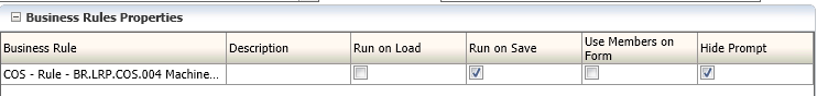
Framework Properties

Abstract Building Blocks

Complete parameterization

Case Study

Abstract Sequence

Generic Script

Parsing Mask

Test Set

Block Mining

Dimensions Analysis

New Simulation Databases

Block Mining Results Query

Dimensions Order Mining

Dimensions Order Mining Results Query

Domain Mining Module

Performance Reports

Sparse Read/Write Relationship

Descriptive statistics

Abstract

In this post we discuss the framework that allows us to perform automated applications optimization, testing, and monitoring. Framework that learns on the past performance and uses its predictions to find the best design and configuration. We will review the framework’s building blocks, and its workflow. Also we’ll use the case study and demonstrate main steps.

Whether you are a business user or a developer, most likely you are constantly reminded that your system needs to be optimized, despite the fact that some efforts were made in the past.

From business point of view optimizing essbase applications is expensive, and time consuming. It consumes not only developer time, but also time of business users. As a result, it is difficult to fit into business cycle.

On a technical side, with the multitude of environment variables that define EPM platforms, tuning essbase applications is not a straight-forward task. Variables impacting performance include compression algorithm, caches allocation, number of CPUs used for task parallelization, alternatives of outline design, underlying infrastructure characteristics, to name just a few.

Moreover, relationship between resources allocation and performance is not linear, resulting in local and sometimes unexpected optimums. The number of combinations is enormous, so testing each one manually is not an option.

How can we find those optimums? We will demonstrate an automated framework that takes user-defined input domains, runs the tests, and streams data to the database for reporting. Still, finding optimal configuration for each environment takes time, but this is mostly machine time. Also, if EPM opens up for collaboration and shares its statistics, the framework can rely more heavily on statistical methods like neural networks with backpropagation, which will allow finding optimal path much faster.

Framework Properties

Abstract Building Blocks

What properties a good performance testing and tuning system should possess? First of all, it should allow a user to easily define a sequence of steps that represents a relevant business process.

In the example of the diagram below, in the first steps we want to configure database settings like Index cache, datacache, commit interval, subvars for calc parallel, calc cache, etc.

Then we reset the database, load level 0 data, run a sequence of calc scripts, and load additional data in between. In the end we want this sequence to be optimized.

In order for the sequence to be easily defined, the building blocks of the sequence need to be generic and abstract.

We would call a generic component (running calc script for example), and pass needed parameters. If you are familiar with ODI, similarly to how we call ODI scenarios from the package and pass parameters, we call generic scripts.

Complete parameterization

Lets present the framework in the form of interacting layers.

We saw that the sequence is constructed of the basic building blocks - generic scripts. They accept parameters from the sequence. However the sequence will need to be executed under many various conditions. For this to happen the sequence itself needs to be fully parameterized. Those conditions can be defined in several layers above the sequence.

Those layers represent modules that generate those conditions automatically, or test sets that can be defined manually by the user. Every layer of the framework should be completely parameterized and be able to inherit parameters from upper layers.

The first layer above Abstract Sequence is the layer of test sets (layer in green). It defines one or more test sets that pass parameters to the sequence. Each set correspond to one execution of the sequence.

Above test sets is a layer of mining modules. They generate test sets dynamically based on the ranges of parameters. The program picks a parameter from each range and passes it to the test set.

There are also specialized mining modules that optimize database structure. They run data analysis, find the best block composition and dimensions order, for example. Again, those modules generate a test set for each simulation which runs an abstract sequence.

What other characteristics the framework should have?

Obviously, logs should be parsed, and relevant statistics should flow automatically into repository. Those will be used in further optimization steps.
The system should be able to learn from prior executions, potentially from other clients as well.
Real-time machine learning/training and real-time feedback into solution search engine.
It shouldn’t depend on a particular operating system
All elements of the framework should be reusable

Workflow

Lets review the workflow diagram at a high level.

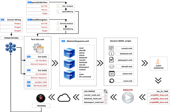
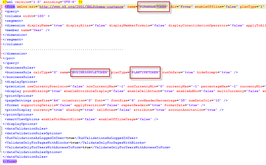
As we saw, at the center is an abstract sequence that represents application life cycle of business process. Each step in it is an XML node that tells which script or command needs to be run, and defines its parameters.
Each node may call a generic and tokenized MAXL script which accepts parameters. In order to execute the script, tokens need to be replaced with values from the abstract sequence. This job is done by the script generator. It produces a set of executable MAXL scripts. Each script corresponds to a step in abstract sequence.
Those scripts are executed and their logs are parsed by a parser. Typically each generic MAXL script has one or more corresponding mask which is used during parsing.
Parsed results are loaded into relational repository.
We saw that one layer above the abstract sequence is a layer of test sets. Each test case defines variables for the abstract sequence it calls. You can define multiple test cases, so that abstract sequence will run multiple times under different conditions.
Test cases can be defined manually, or they can accept variables permutations from one level above - a level of mining modules.
That level could be a block mining module, which analyzes dimensions structure, data density, and as a result generates a set of databases for simulations. Each database has a different set of dense dimensions. So the block mining module creates multiple test sets, and each test set is run on a different database.
Similarly to block mining module, order mining module gets the best block composition from block mining module and generates multiple databases with the same block composition, but different orderings of sparse dimensions. The module uses common heuristics for sparse dimensions ordering, such as Parent/Child ratio, dimension density, dimension size, and non-aggregating dimensions placement.
Finally, domain mining module defines the ranges of database settings, or any abstract sequence parameter. For example, it could be database index and data caches. A range of 10M to 500M for index and a range of 100K to 4Gb for data cache. It could also be a range of threads used in the calculation - between 1 and 8, or task dimensions.

Here we should pause for a second and reflect. We could potentially have dozens of ranges, each one having multiple values. The number of possible permutations of those parameters could be astronomical. For instance, if we have 10 domains, each having 10 possible values, the total number of permutations is 10^10, or 10 billion. If we try to run our sequence for every possible combination, and on average it takes 20 min to complete the sequence, it’ll take us 380,000 years until optimization is done. In consulting terms it’s a really long term engagement.

This means we cannot crawl through all possible permutations, but have to run only promising combinations that potentially lead to optimum. At the high level we can achieve this by separating independent variables or clusters of independent variables first. For example the optimal value of the index cache will depend on the size of the index file, and can be optimized in the end, independently. Commit interval, calculator cache and data cache are related and can be optimized as a separate cluster of variables.

On the other hand, if we have large enough result set of past executions, we can employ statistical methods to predict optimal values and test those hypothesis.

Either way, while choosing the next iteration, the system should incorporate the knowledge about the past iterations on the same or other systems.

Case Study

Abstract Sequence

In our demo the first 2 things we want our framework to find are the optimal block composition and sparse dimensions order. We start by defining the abstract sequence. We assume that the outline was already built and data loaded.

It is a basic sequence of loading the data, running complete aggregation and reset.

<?xml version="1.0" encoding="ISO-8859-1"?>

</STEP>

</STEP>

</STEP>

</STEP>

</STEP>

</STEP>

</STEP>

<VAR10><![CDATA['/<WAPP>/<WDB>/DataH.txt']]></VAR10>

</STEP>

<VAR10><![CDATA['/<WAPP>/<WDB>/DataH_1.txt']]></VAR10>

</STEP>

</STEP>

</STEP>

</SEQUENCE>

In the first steps we set Index cahce, data cache, and commit interval. As you can see all these step call the same alterdb.msh.

Generic Script

This is how alterdb.msh looks like.

spool on to <VAR4>;

set column_width 100;

set timestamp on;

alter application <VAR5> load database <VAR6>;

alter database <VAR5>.<VAR6> unlock all objects;

alter database <VAR5>.<VAR6> set <VAR7> <VAR8> <VAR9>;

alter database <VAR5>.<VAR6> disable autostartup;

alter system unload application <VAR5>;

alter system load application <VAR5>;

query database <VAR5>.<VAR6> get dbstats dimension;

query database <VAR5>.<VAR6> get dbstats data_block;

logout;

spool off;

It contains alter database parameterized statements. Then application is restarted, and database statistics are queried. You usually don’t have to change the msh file since VAR tokens provide enough flexibility. And values for those tokens are passed from the abstract sequence.

You can see that many values in abstract sequence parameterized (there are angle brackets around them). The values for those come either from test set, like application name and database name, or global variables such as essbase server. In fact values can come from any of the upper layer.

After all tokens in angle brackets are replaced we end up with the file similar to this one, which can be executed with msh.

spool on to D:\\AutomationsV2\\TetsSets\\xxx\\TEMPMAXL\\alterdb._SetEADO01._0_1431550126_1431550224129.log;

set column_width 100;

set timestamp on;

alter application TST_EA load database EADO_B8;

alter database TST_EA.EADO_B8 unlock all objects;

alter database TST_EA.EADO_B8 set index_cache_size 50000000 ;

alter database TST_EA.EADO_B8 disable autostartup;

alter system unload application TST_EA;

alter system load application TST_EA;

query database TST_EA.EADO_B8 get dbstats dimension;

query database TST_EA.EADO_B8 get dbstats data_block;

logout;

spool off;

Lets get back to our sequence. The next steps define substitution variables. Subvars such as the number of CPUs in CALCPARALLEL statement, or the size of calculator cache. Those can also be member names, or any value used in calculation scripts.

And this is the calc script itself.

//ESS_LOCALE English_UnitedStates.Latin1@Binary

SET CACHE ALL;

SET CACHE &PT_CACHE;

SET CALCPARALLEL &PT_CALCPARALLEL1;

SET MSG SUMMARY;

SET AGGMISSG ON;

FIX (@relative(TimePeriod,0),@LEVMBRS("Scenario",0), @LEVMBRS("Version",0),@LEVMBRS("Year",0),@Descendants(Entity),@relative("Account",0))

FIX (@LEVMBRS("View",0),@relative("HFM Value",0))

AGG("CostCenter","PCC","Intercompany Partner");

ENDFIX;

You can see that Calculator cache is also set up via the subvar and optimization framework.

Then we have data load, run calculation a reset statement. Data load command can take any form allowed by MAXL.

Parsing Mask

You can notice LOGMASK property of XML node. This is the file that defines what properties we want to collect from the log file. In case of runcalc we want to collect elapsed time, blocks created, dense and sparse reads and writes, etc.

<?xml version="1.0" encoding="ISO-8859-1"?>

<STEPTIME><![CDATA[Total Calc Elapsed Time for [<CALCFILE>] : [<STATVALUE>] seconds.]]></STEPTIME>

<TOTALBLOCKSCREATED><![CDATA[Total Block Created: [<STATVALUE>] Blocks]]></TOTALBLOCKSCREATED>

<SPARSEREAD><![CDATA[Sparse Calculations: [<SPARSEWRITE>] Writes and [<STATVALUE>] Reads]]></SPARSEREAD>

<DENSEWRITE><![CDATA[Dense Calculations: [<STATVALUE>] Writes]]></DENSEWRITE>

<DENSEREAD><![CDATA[Dense Calculations: [<DENSEWRITE>] Writes and [<STATVALUE>] Reads]]></DENSEREAD>

<SPARCECELLS><![CDATA[Sparse Calculations: [<STATVALUE>] Cells]]></SPARCECELLS>

<DENSECELLS><![CDATA[Dense Calculations: [<STATVALUE>] Cells]]></DENSECELLS>

</SET>

</sequence>

So this is our sequence. Now we need to define a test set that will pass parameters like DATACACHE, COMMITAFTER and others. Those that are in angle brackets.

Test Set

And this is our test set. It contains a single test case.

<?xml version="1.0" encoding="ISO-8859-1"?>

<PT_CALCPARALLEL1><![CDATA['3']]></PT_CALCPARALLEL1>

<PT_CALCPARALLEL2><![CDATA['3']]></PT_CALCPARALLEL2>

<PT_CALCPARALLEL3><![CDATA['3']]></PT_CALCPARALLEL3>

<PT_CALCPARALLEL4><![CDATA['3']]></PT_CALCPARALLEL4>

<PT_CALCPARALLEL5><![CDATA['3']]></PT_CALCPARALLEL5>

<PT_CALCPARALLEL6><![CDATA['3']]></PT_CALCPARALLEL6>

<PT_CALCPARALLEL7><![CDATA['3']]></PT_CALCPARALLEL7>

<PT_CACHE><![CDATA['DEFAULT']]></PT_CACHE>

<PT_CALCTASKDIMS1><![CDATA['3']]></PT_CALCTASKDIMS1>

<PT_CALCTASKDIMS2><![CDATA['3']]></PT_CALCTASKDIMS2>

<PT_CALCTASKDIMS3><![CDATA['3']]></PT_CALCTASKDIMS3>

<PT_CALCTASKDIMS4><![CDATA['3']]></PT_CALCTASKDIMS4>

<PT_CALCTASKDIMS5><![CDATA['3']]></PT_CALCTASKDIMS5>

<PT_CALCTASKDIMS6><![CDATA['3']]></PT_CALCTASKDIMS6>

<PT_CALCTASKDIMS7><![CDATA['3']]></PT_CALCTASKDIMS7>

</SET>

</sequence>

You can see that most of the parameters are hardcoded, since in this example we are interested in finding the optimal block composition. So it wouldn’t make sense to change cache sizes, or number of threads in calculation, at the same time.

The only variable parameters are application name, database name, and description. Block mining module will create new databases and will run abstract sequence on each one of them.

Notice ABSTRACT property: it references the name of the abstract sequence into which it is going to pass its parameters. This is how a TEST SET is tied with an abstract sequence.

Block Mining

Finally, lets define the block mining properties. This is done in another XML file, in one layer above the test set.

<?xml version="1.0" encoding="ISO-8859-1"?>

<SET>

</SET>

</sequence>

Here we define the source app and source cube: it is going to be used as a source for replication. Target cube - is a prefix used in target cubes. In this example the prefix is EABM, so database names will be EABM0, EABM1,2,3, etc.

Another setting is BLOCKMININGTHRESHOLD. We said that in order to find the best block composition the program will create new databases and will run simulation sequence. However it will not pick up dimensions randomly. It will do the dimension density analysis first, and will add to block, combinations of dimensions with densities above certain threshold. So this is dimension density threshold.

One exception to this rule is account dimension. It will be present in the block regardless of its dimension density.

We have a few options how to run the framework. We can run it step by step, so that we can examine results in the end of each step, or we can run end-to-end optimization. In this presentation we will run it step by step.

So the first step is block mining. We pass two parameters: startup.xml file with high level parameters, and blockmining keyword.

stratup.xml contains high level parameters like PARAMFILE, and reference to the BlockMiningEA01.xml that we just defined. It also contains references to other mining module like DOMAINMAP and DIMORDERMAP. We will define those in the next steps.

<?xml version="1.0" encoding="ISO-8859-1"?>

<SET>

</SET>

</sequence>

Dimensions Analysis

The first thing the block mining module does is dimension analysis. The results are output into this file.

Dense dimension: Account

ActualSize: 1424.0

ActualSizeFlatInEnd: 1424.0

blockDensity: 0.9337298215802888

parentChildRatio: 0.18047752808988765

parenChildFlatInEnd: 0.18047752808988765

densityFlatInEnd: 0.9337298215802888

bottomLevelCounter: 1167.0

ActualMaxBlocks: 4.5202355224879104E17

actualBlockSize: 1177

ActualBlockSizeFlatInEnd: 1177

declaredBlockSize: 1487

getCompressionRatio: 0.02172849915682968

getDeclaredMaxBlocks: 3.8331796781431296E18

getPagedInBlocks: 0.0

getPerformanceStatistics:

getTotalBlocks: 8495239.0

---------------------------------------

Dense dimension: TimePeriod

ActualSize: 18.0

ActualSizeFlatInEnd: 18.0

blockDensity: 33.0

parentChildRatio: 0.2777777777777778

parenChildFlatInEnd: 0.2777777777777778

densityFlatInEnd: 33.0

bottomLevelCounter: 13.0

ActualMaxBlocks: 3.5760085466793247E19

actualBlockSize: 13

ActualBlockSizeFlatInEnd: 13

declaredBlockSize: 19

getCompressionRatio: 0.6504545454545455

getDeclaredMaxBlocks: 2.999967463894123E20

getPagedInBlocks: 0.0

getPerformanceStatistics:

getTotalBlocks: 1.4968137E7

---------------------------------------

Dense dimension: Version

ActualSize: 12.0

ActualSizeFlatInEnd: 1.0E9

blockDensity: 8.333333333333332

parentChildRatio: 0.0

parenChildFlatInEnd: 100.0

densityFlatInEnd: 100.0

bottomLevelCounter: 12.0

ActualMaxBlocks: 5.364012820018987E19

actualBlockSize: 12

ActualBlockSizeFlatInEnd: 12

declaredBlockSize: 13

getCompressionRatio: 0.5238095238095238

getDeclaredMaxBlocks: 4.3845678318452566E20

getPagedInBlocks: 0.0

getPerformanceStatistics:

getTotalBlocks: 6.3370293E7

---------------------------------------

Dense dimension: BusinessUnit

ActualSize: 138.0

ActualSizeFlatInEnd: 138.0

blockDensity: 1.2658227848101267

parentChildRatio: 0.43478260869565216

parenChildFlatInEnd: 0.43478260869565216

densityFlatInEnd: 1.2658227848101267

bottomLevelCounter: 78.0

ActualMaxBlocks: 4.6643589739295539E18

actualBlockSize: 79

ActualBlockSizeFlatInEnd: 79

declaredBlockSize: 291

getCompressionRatio: 0.125

getDeclaredMaxBlocks: 1.9587416430923825E19

getPagedInBlocks: 0.0

getPerformanceStatistics:

getTotalBlocks: 5.4541355E7

---------------------------------------

Dense dimension: Scenario

ActualSize: 19.0

ActualSizeFlatInEnd: 1.0E9

blockDensity: 5.263157894736842

parentChildRatio: 0.0

parenChildFlatInEnd: 100.0

densityFlatInEnd: 100.0

bottomLevelCounter: 19.0

ActualMaxBlocks: 3.3877975705383076E19

actualBlockSize: 19

ActualBlockSizeFlatInEnd: 19

declaredBlockSize: 20

getCompressionRatio: 0.39285714285714285

getDeclaredMaxBlocks: 2.8499690906994167E20

getPagedInBlocks: 0.0

getPerformanceStatistics:

getTotalBlocks: 6.3370293E7

---------------------------------------

Dense dimension: View

ActualSize: 2.0

ActualSizeFlatInEnd: 1.0E9

blockDensity: 100.0

parentChildRatio: 0.0

parenChildFlatInEnd: 100.0

densityFlatInEnd: 100.0

bottomLevelCounter: 2.0

ActualMaxBlocks: 3.218407692011392E20

actualBlockSize: 2

ActualBlockSizeFlatInEnd: 2

declaredBlockSize: 3

getCompressionRatio: 1.0

getDeclaredMaxBlocks: 1.8999793937996112E21

getPagedInBlocks: 0.0

getPerformanceStatistics:

getTotalBlocks: 3.7053516E7

---------------------------------------

Dense dimension: Year

ActualSize: 17.0

ActualSizeFlatInEnd: 1.0E9

blockDensity: 5.88235294117647

parentChildRatio: 0.0

parenChildFlatInEnd: 100.0

densityFlatInEnd: 100.0

bottomLevelCounter: 17.0

ActualMaxBlocks: 3.786361990601638E19

actualBlockSize: 17

ActualBlockSizeFlatInEnd: 17

declaredBlockSize: 18

getCompressionRatio: 0.43038461538461537

getDeclaredMaxBlocks: 3.166632322999352E20

getPagedInBlocks: 0.0

getPerformanceStatistics:

getTotalBlocks: 4.6809998E7

---------------------------------------

Dense dimension: PCC

ActualSize: 98.0

ActualSizeFlatInEnd: 98.0

blockDensity: 1.3673469387755102

parentChildRatio: 0.25510204081632654

parenChildFlatInEnd: 0.25510204081632654

densityFlatInEnd: 1.3673469387755102

bottomLevelCounter: 73.0

ActualMaxBlocks: 6.5681789632885555E18

actualBlockSize: 98

ActualBlockSizeFlatInEnd: 98

declaredBlockSize: 99

getCompressionRatio: 0.10663551401869159

getDeclaredMaxBlocks: 5.757513314544276E19

getPagedInBlocks: 0.0

getPerformanceStatistics:

getTotalBlocks: 3.103252E7

---------------------------------------

Dense dimension: Intercompany Partner

ActualSize: 60.0

ActualSizeFlatInEnd: 60.0

blockDensity: 1.6666666666666667

parentChildRatio: 0.05

parenChildFlatInEnd: 0.05

densityFlatInEnd: 1.6666666666666667

bottomLevelCounter: 57.0

ActualMaxBlocks: 1.0728025640037974E19

actualBlockSize: 60

ActualBlockSizeFlatInEnd: 60

declaredBlockSize: 60

getCompressionRatio: 0.15942028985507245

getDeclaredMaxBlocks: 9.499896968998057E19

getPagedInBlocks: 0.0

getPerformanceStatistics:

getTotalBlocks: 6.3238266E7

---------------------------------------

Dense dimension: HFM Value

ActualSize: 64.0

ActualSizeFlatInEnd: 64.0

blockDensity: 2.822222222222222

parentChildRatio: 0.3125

parenChildFlatInEnd: 0.3125

densityFlatInEnd: 2.822222222222222

bottomLevelCounter: 44.0

ActualMaxBlocks: 1.00575240375356E19

actualBlockSize: 45

ActualBlockSizeFlatInEnd: 45

declaredBlockSize: 64

getCompressionRatio: 0.2087037037037037

getDeclaredMaxBlocks: 8.906153408435678E19

getPagedInBlocks: 0.0

getPerformanceStatistics:

getTotalBlocks: 3.7721755E7

---------------------------------------

Dense dimension: Entity

ActualSize: 87.0

ActualSizeFlatInEnd: 87.0

blockDensity: 4.540229885057472

parentChildRatio: 0.3333333333333333

parenChildFlatInEnd: 0.3333333333333333

densityFlatInEnd: 4.540229885057472

bottomLevelCounter: 58.0

ActualMaxBlocks: 7.3986383724399821E18

actualBlockSize: 87

ActualBlockSizeFlatInEnd: 87

declaredBlockSize: 87

getCompressionRatio: 0.1553125

getDeclaredMaxBlocks: 6.551653082067625E19

getPagedInBlocks: 0.0

getPerformanceStatistics:

getTotalBlocks: 1.3823985E7

---------------------------------------

Dense dimension: CostCenter

ActualSize: 717.0

ActualSizeFlatInEnd: 717.0

blockDensity: 0.15151515151515152

parentChildRatio: 0.33751743375174337

parenChildFlatInEnd: 0.33751743375174337

densityFlatInEnd: 0.15151515151515152

bottomLevelCounter: 475.0

ActualMaxBlocks: 8.9774273138393088E17

actualBlockSize: 660

ActualBlockSizeFlatInEnd: 660

declaredBlockSize: 1493

getCompressionRatio: 0.016442451420029897

getDeclaredMaxBlocks: 3.8177750712651264E18

getPagedInBlocks: 0.0

getPerformanceStatistics:

getTotalBlocks: 1.694099E7

---------------------------------------

Different dimensions statistics are used in finding the best block composition or dimensions order. For example we use block density to identify which dimension it would make sense to add to the block.

We also gather statistics like parentChildRatio, ActualSize which will be used by other modules.

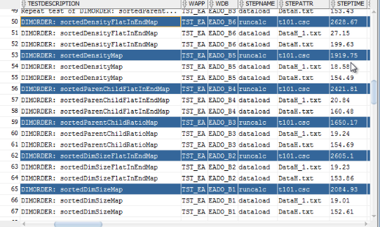
New Simulation Databases

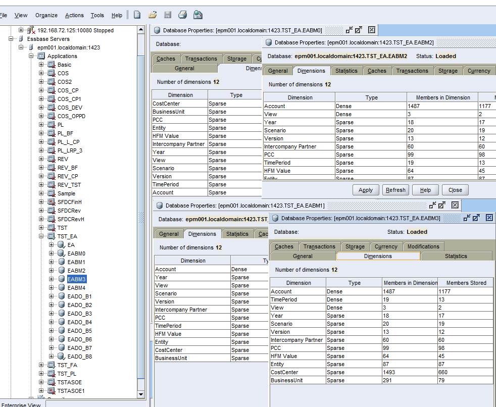
You can see that new databases were added to application: EABM0 to 4. Whereas EA is our source application.

Lets take a look at the properties of those databases.

Account is a default dense dimension always present in the block. 3 other databases are addition of either View, TimePeriod, or both dimensions. Why don’t we add other dimensions to the block? Because we set a threshold in BlockMining definition file to 10%.

Now lets see what files where generated by the framework. Lets have a look at this one - delayedBlockMiningSets.

D:\\AutomationsV2\\TetsSets\\Kscope15\\TEMPMAXL\\SetEABM01._0_TST_EA_EABM1_1431475416.bat

D:\\AutomationsV2\\TetsSets\\Kscope15\\TEMPMAXL\\SetEABM01._0_TST_EA_EABM2_1431475416.bat

D:\\AutomationsV2\\TetsSets\\Kscope15\\TEMPMAXL\\SetEABM01._0_TST_EA_EABM3_1431475416.bat

D:\\AutomationsV2\\TetsSets\\Kscope15\\TEMPMAXL\\SetEABM01._0_TST_EA_EABM4_1431475416.bat

There are 4 batch files in it. Each corresponds to a new database. Lets open one of them.

call startMaxl.cmd D:\\AutomationsV2\\TetsSets\\Kscope15\\TEMPMAXL\\alterdb._SetEABM01._0_1431475416_1431495155280.msh

call startMaxl.cmd D:\\AutomationsV2\\TetsSets\\Kscope15\\TEMPMAXL\\alterdb._SetEABM01._0_1431475416_1431495155297.msh

call startMaxl.cmd D:\\AutomationsV2\\TetsSets\\Kscope15\\TEMPMAXL\\alterdb._SetEABM01._0_1431475416_1431495155301.msh

call startMaxl.cmd D:\\AutomationsV2\\TetsSets\\Kscope15\\TEMPMAXL\\setvar._SetEABM01._0_1431475416_1431495155305.msh

call startMaxl.cmd D:\\AutomationsV2\\TetsSets\\Kscope15\\TEMPMAXL\\setvar._SetEABM01._0_1431475416_1431495155309.msh

call startMaxl.cmd D:\\AutomationsV2\\TetsSets\\Kscope15\\TEMPMAXL\\setvar._SetEABM01._0_1431475416_1431495155317.msh

call startMaxl.cmd D:\\AutomationsV2\\TetsSets\\Kscope15\\TEMPMAXL\\setvar._SetEABM01._0_1431475416_1431495155321.msh

call startMaxl.cmd D:\\AutomationsV2\\TetsSets\\Kscope15\\TEMPMAXL\\dataload._SetEABM01._0_1431475416_1431495155326.msh

call startMaxl.cmd D:\\AutomationsV2\\TetsSets\\Kscope15\\TEMPMAXL\\dataload._SetEABM01._0_1431475416_1431495155330.msh

call startMaxl.cmd D:\\AutomationsV2\\TetsSets\\Kscope15\\TEMPMAXL\\runcalc._SetEABM01._0_1431475416_1431495155334.msh

call startMaxl.cmd D:\\AutomationsV2\\TetsSets\\Kscope15\\TEMPMAXL\\reset._SetEABM01._0_1431475416_1431495155339.msh

We see that a sequence of msh files is executed. a few alterdb files, setvers, then dataload, runcalc, and reset. You realize that each file here corresponds to an XML node in our abstract sequence. So this file is a representation of a single test case from a test set.

Block Mining Results Query

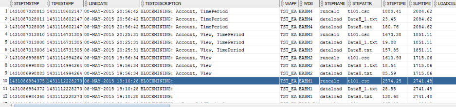
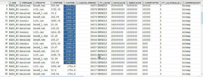
Lets run this test set and see what happens. Here is the summary execution results.

SUMTIME column tells you what was the total length of the sequence, and STEPTIME gives you the execution time of individual step.

TEST DESCRIPTION provides details about block composition within a particular simulation.

The first simulation was for block consisting of only Account dimension. And it took 2741 sec. The longest step was runcalc t101 which took 2574 sec.

Then View dimension was added, and sequence time dropped to 1715 sec.

Then TimePeriod was added, which added 136 sec.

And finally, a Account and TimePeriod were left in the block, and View removed. This added 233 sec.

So we have 2 candidates for block composition: Account and View (the best sequence time) and Account, View, TimePeriod, which is 8% slower.

If the program is allowed to choose block composition automatically, it would choose a block composed of Account and View dimensions. But in our sequence we did not add retrieval simulations. And we know that TimePeriod is dynamic dimension, so keeping it dynamic and outside of a block would impact retrieval time. So we could either add retrieval simulation to the sequence, or intervene and choose a block with TimePeriod in it. That’s what we would do in this demo.

Dimensions Order Mining

The next phase of our optimization is finding optimal dimensions order. Similarly to block mining XML we have dimensions order mining definition XML file. It also has a source cube property. Here we update the file manually with EABM3, since that’s the database with block consisting of 3 dimensions: Account, View and TimePeriods. Remember that we may need to update this file only if we want to interfere with automatic process of the best block composition.

<?xml version="1.0" encoding="ISO-8859-1"?>

<SET>

</SET>

</sequence>

Target cube - that is placeholder for automatically generated cubes.

DIMORDERMININGDENSITYFILE property points to a file that contains density, parent/child ratio, and other statistics for each dimension.

Dimensions Order Mining Results Query

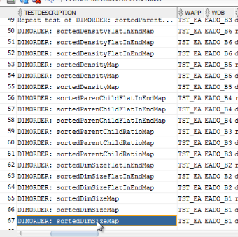
Lets run the dimOrder process and see the results.

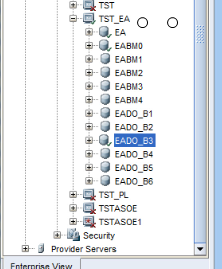
You can see that the process created 6 new databases - each corresponding to one of the ordering methodologies.

Lets take a look at database properties. From test description you can see, that the type of ordering for the first database is Dimension size.

The next one is Dimension size with flat dimensions in the end. This is actual dimension size, including dynamic members. There are another 2 orderings that take into account only stored members. Then we have ordering based on parent/child ratio, and dimension density.

If we check the execution times of individual steps or the total sequence time, we see that ordering based on parent/child ratio gives the best results.

Since we have candidates for the best block definition and dimensions ordering, we can move on to defining the best database settings, or calculation options. This is done by running domain mining module.

Domain Mining Module

Lets start with 3 parameters: CALCCACHE,DATACACHE and COMMITAFTER. We define range for each one, and the granularity.

<?xml version="1.0" encoding="ISO-8859-1"?>

<SET>

</SET>

</sequence>

The first 2 parameters define beginning and the end of the range, and the third one into how many segments the range is divided. The default is 2. So we will have 3 values from the range: beginning, middle, and the end. If we define granularity of 5, we will have 6 values, and so on.

Once we run the module, similarly to block mining and order mining modules the program generates a file with all the test sets.

D:\\AutomationsV2\\TetsSets\\Kscope15\\TEMPMAXL\\SetEADM02._1__1431454752.bat

D:\\AutomationsV2\\TetsSets\\Kscope15\\TEMPMAXL\\SetEADM02._2__1431454752.bat

D:\\AutomationsV2\\TetsSets\\Kscope15\\TEMPMAXL\\SetEADM02._3__1431454752.bat

D:\\AutomationsV2\\TetsSets\\Kscope15\\TEMPMAXL\\SetEADM02._4__1431454752.bat

D:\\AutomationsV2\\TetsSets\\Kscope15\\TEMPMAXL\\SetEADM02._5__1431454752.bat

D:\\AutomationsV2\\TetsSets\\Kscope15\\TEMPMAXL\\SetEADM02._6__1431454752.bat

D:\\AutomationsV2\\TetsSets\\Kscope15\\TEMPMAXL\\SetEADM02._7__1431454752.bat

D:\\AutomationsV2\\TetsSets\\Kscope15\\TEMPMAXL\\SetEADM02._8__1431454752.bat

D:\\AutomationsV2\\TetsSets\\Kscope15\\TEMPMAXL\\SetEADM02._9__1431454752.bat

D:\\AutomationsV2\\TetsSets\\Kscope15\\TEMPMAXL\\SetEADM02._10__1431454752.bat

D:\\AutomationsV2\\TetsSets\\Kscope15\\TEMPMAXL\\SetEADM02._11__1431454752.bat

D:\\AutomationsV2\\TetsSets\\Kscope15\\TEMPMAXL\\SetEADM02._12__1431454752.bat

D:\\AutomationsV2\\TetsSets\\Kscope15\\TEMPMAXL\\SetEADM02._13__1431454752.bat

D:\\AutomationsV2\\TetsSets\\Kscope15\\TEMPMAXL\\SetEADM02._14__1431454752.bat

D:\\AutomationsV2\\TetsSets\\Kscope15\\TEMPMAXL\\SetEADM02._15__1431454752.bat

D:\\AutomationsV2\\TetsSets\\Kscope15\\TEMPMAXL\\SetEADM02._16__1431454752.bat

D:\\AutomationsV2\\TetsSets\\Kscope15\\TEMPMAXL\\SetEADM02._17__1431454752.bat

D:\\AutomationsV2\\TetsSets\\Kscope15\\TEMPMAXL\\SetEADM02._18__1431454752.bat

D:\\AutomationsV2\\TetsSets\\Kscope15\\TEMPMAXL\\SetEADM02._19__1431454752.bat

D:\\AutomationsV2\\TetsSets\\Kscope15\\TEMPMAXL\\SetEADM02._20__1431454752.bat

D:\\AutomationsV2\\TetsSets\\Kscope15\\TEMPMAXL\\SetEADM02._21__1431454752.bat

D:\\AutomationsV2\\TetsSets\\Kscope15\\TEMPMAXL\\SetEADM02._22__1431454752.bat

D:\\AutomationsV2\\TetsSets\\Kscope15\\TEMPMAXL\\SetEADM02._23__1431454752.bat

D:\\AutomationsV2\\TetsSets\\Kscope15\\TEMPMAXL\\SetEADM02._24__1431454752.bat

D:\\AutomationsV2\\TetsSets\\Kscope15\\TEMPMAXL\\SetEADM02._25__1431454752.bat

D:\\AutomationsV2\\TetsSets\\Kscope15\\TEMPMAXL\\SetEADM02._26__1431454752.bat

D:\\AutomationsV2\\TetsSets\\Kscope15\\TEMPMAXL\\SetEADM02._27__1431454752.bat

SELFTUNE 1431454752

You can notice that in the end we also have a parameter SELFTUNE 1431454752, whereas in the domain definition we have property DOMAINDSELFTUNE. It means that after the program finishes running 27 sequences, for all possible values from the domain, it will start self-tuning process, which will create additional test sets, based on the results of the domain execution.

The results are written into repository, and you can see changing parameters in the summary view.

Performance Reports

So far we saw the main steps controlling the process. They created many data points, now we may need to present them in a meaningful fashion to IT department or implementing partner, and to stakeholders, making decisions about the future of Hyperion systems.

They would need to decide whether to invest into hardware, or making changes to systems’ architecture.

Lets see how this report may look like. The report we are going to see is based on different data sets and hardware, so the numbers are slightly different from what we saw in previous slides.

In the report we present findings of each step. Here are dimension statistics, and description of the tests designed to find best block composition.

Dense dimension	Size	Density	P/C Ratio	P/C FIE	Density FIE	Compression
View	3	66.67	0.33	100	100	1
TimePeriod	18	33	0.28	0.28	33	0.65
Version	13	7.69	0.08	100	100	0.5
Year	18	5.56	0.06	100	100	0.42
Scenario	20	5	0.05	100	100	0.38
Entity	87	4.54	0.33	0.33	4.54	0.16
HFM Value	64	2.82	0.31	0.31	2.82	0.21
Intercompany Partner	60	1.67	0.05	0.05	1.67	0.16
PCC	98	1.37	0.26	0.26	1.37	0.11
BusinessUnit	138	1.27	0.43	0.43	1.27	0.13
Account	1424	0.93	0.18	0.18	0.93	0.02
CostCenter	717	0.15	0.34	0.34	0.15	0.02

Block mining results, impact of each step in the sequence and candidates for best composition.

	ODIClear.csc	ODIAgg.csc	AggAll.csc	DataH_1.txt	DataH.txt	Total
Account, View, Version	4.54	2.37	5962.21	89.87	386.11	6445.1
Account, TimePeriod, Version	1.88	2.81	14246.5	158.63	1299.26	15709.08
Account, TimePeriod	1.84	2.37	1801.76	25.15	198.69	2029.81
Account, View, TimePeriod, Version	1.71	2.62	16286.7	156.34	1356.82	17804.19
Account, View, TimePeriod	1.62	2.07	1663.12	22.48	164.78	1854.07
Account, View	4.63	2.16	1992.07	21.89	113.98	2134.73
Account	5.13	5.31	3351.27	32.07	149.78	3543.56

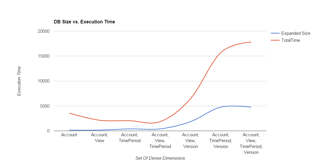
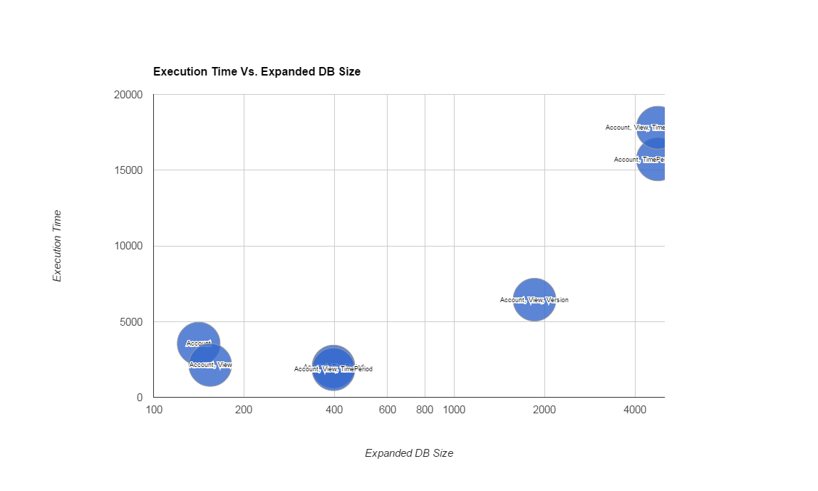
We may want to do additional analysis based on the data we collected. For example relationship between expanded database size and execution time.

We see for example that the smallest database size does not necessarily mean the best performance.

The same mining process can be run on a different hardware, or on a hardware under stress, with limited resources.

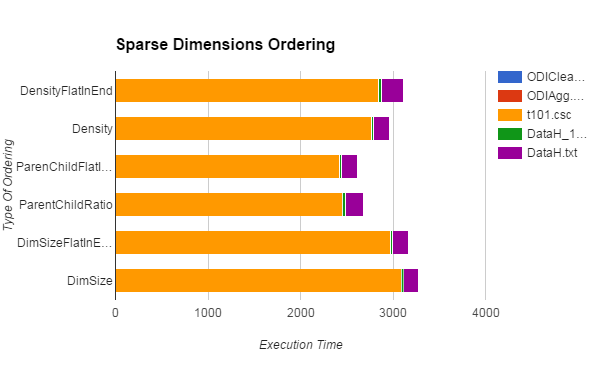
Similar report for dimensions ordering, relationship between the total number of reads/writes and execution time.

	ODIClear.csc	ODIAgg.csc	t101.csc	DataH_1.txt	DataH.txt	Total
DensityFlatInEnd	0	0.25	2841.68	33.94	236.98	3112.85
Density	1.35	2.37	2766.05	21.79	165.28	2956.84
ParenChildFlatInEnd	0	0.37	2423.84	23.07	165.88	2613.16
ParentChildRatio	1.61	2.04	2448.96	28.81	196.62	2678.04
DimSizeFlatInEnd	0	0.05	2977.59	21.49	166.35	3165.48
DimSize	2.66	2.07	3085.4	22.65	167.83	3280.61

Sparse Read/Write Relationship

	SPARSEWRITE x 10^-4	SPARSEREAD x 10^-4	SUMTIME
DimSize	1094.8	2606.7	3280.61
DimSizeFlatInEnd	1093.9	2476.5	3165.48
ParentChildRatio	1094.8	2480.6	2678.04
ParenChildFlatInEnd	1094.3	2479.3	2613.16
Density	1094.8	2895.7	2956.84
DensityFlatInEnd	1094.8	3040.5	3112.85

You can see that the total number of writes is the same for all orderings. This is expected, since we need to calculate the same number of blocks regardless of the dimensions order. The number of reads however, does depends on the dimensions order. We see that the execution time correlates with the number of reads, but variability is not fully explained by it.

We could run order mining simulations for a few block composition candidates. We do that by defining different source database in XML definition file.

Once we run domain mining module we could examine patterns of execution time variability as a result of changing range parameters.

Descriptive statistics

The minimum execution time is 2548.18.

The maximum execution time is 3383.7.

The max-min difference is 835 sec - 33% of the minimum.

The graph above shows that at the low DATACACHE levels spikes in CALCCACHE correspond to dips in SUMTIME. At the higher DATACACHE levels relationship disappears.

Execution time deeps in the middle of CALCCACHE range.

Here for example you can notice that at the low DATACACHE levels, spikes in CALCCACHE correspond to dips in total TIME. At the higher DATACACHE levels this relationship disappears.

With 3D graphs shown here we may want to show trends in execution time. Finding those trends manually is not required though, since self-tuning algorithm finds them automatically and adjusts parameters as needed. One exception is calculator cache. The values that calc cache can accept are discontinuous. It can be LOW, DEFAULT and HIGH. On the other hand numeric value is assigned in essbase configuration file, and essbase server needs to be restarted. So in those cases, if you want to fine-tune the value of calculator cache, you would need to find the trend, and adjust the value in config file manually.

By the way, these graphs are generated automatically, so you shouldn’t be concerned about amount of work required to create them.

Lets take a look at some relationships.

Datacache:200MB		COMMIT	x10^-2
ExecTime-2,500 sec		30	515	1000
CALCCACHEx10^-5	50	622.69	627.43	482.14
	500	444.45	247.8	296.99
	2000	159.83	121.77	106.34

Trend:

Decreasing execution time as a result of increasing commit interval or calculator cache. For mid-level calc cache best performance achieved at mid-level commit interval (there’s a deep in the middle of the plane).

Further tests:

Expand commit boundary. Calc cache increase is not possible, as it reached the maximum of 200MB.

COMMIT: 100K-300K.

CALCCACHE: 200MB

DATACACHE:200MB

Here we see that at low levels of data cache the best performance is achieved with high calc cache and high commit interval. We cannot increase calc cache above 200MB, so we can run additional tests at higher values of commit interval.

This is a consistent trend for LOW, DEFAULT and HIGH values of calc cache so these tests would be automatically added by self-tuning algorithm.

We see a different situation at the datacache of 1.6gb. The best performance is achieved at the mid-level calc cache.

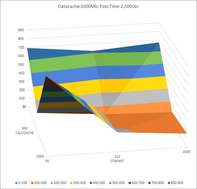
Datacache:1,600MB		COMMIT	x10^-2
ExecTime-2,500 sec		30	515	1000
CALCCACHEx10^-5	50	692.95	615.32	671.78
	500	204.82	141.54	115.55
	2000	883.7	216.62	153.16

Trends

The best performance is at mid-level calc cache.
Increasing commit interval leads to better performance in mid-high levels of calc cache.
Poor performance at low levels of calc cache.

Further tests:

COMMIT: 100K-300K.
CALCCACHE: 30MB-60MB

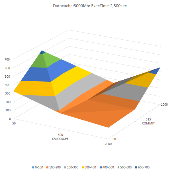
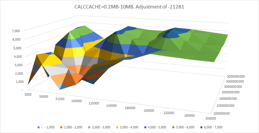
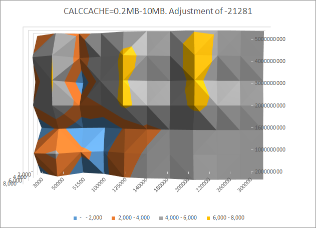
And if we increase data cache even further the best performance is at low calc cache of 5MB.

Datacache:3,000MB		COMMIT	x10^-2
ExecTime-2,500 sec		30	515	1000
CALCCACHEx10^-5	50	325.91	626.05	48.18
	500	180.15	142.54	153.85
	2000	131.53	142.46	451.82

Trends

At 3,000MB level of datacache neither commit interval increment or calc cache increment lead to monotonic performance improvement.
The best performance results are at the corners of the plane at CALCCACHE 200Mb: COMMIT 3000, and CALCCACHE 5Mb: COMMIT 100,000

Further tests

Test 1:

COMMIT: 100K-300K.
CALCCACHE: 0.2MB-10MB

Test 2:

COMMIT: 1000-5000.
CALCCACHE: 200MB

If our sequence takes a long time to ran, we can reduce the data set by deleting the data from one of the non-aggregating dimensions, a year for example. Running tests on a data set of one year instead of 5 years should produce the same results.

What if we want to use results from tests that ran on 5 years and 1 year? Obviously we cannot use total time, since it would be 5 times higher. We can introduce a new metric though. And that would be the ratio of number of loaded cells to total execution time. It will indicate how many cells our sequence is capable to process per second. The higher that number - the better. That means our test runs faster. So we would want to maximize that ratio.

Remember that originally we ran our tests for all combinations defined by the range and granularity. If for example we have 2 domains: commit interval and data cache, with default granularity, we will have 3 values for each domain, and 9 test sets.

When self tuning algorithm analyzes results it may expand the boundaries of the range and increase granularity. But it will run tests only for a subset of possible combinations. It will run only those combinations, that are expected to give better results.

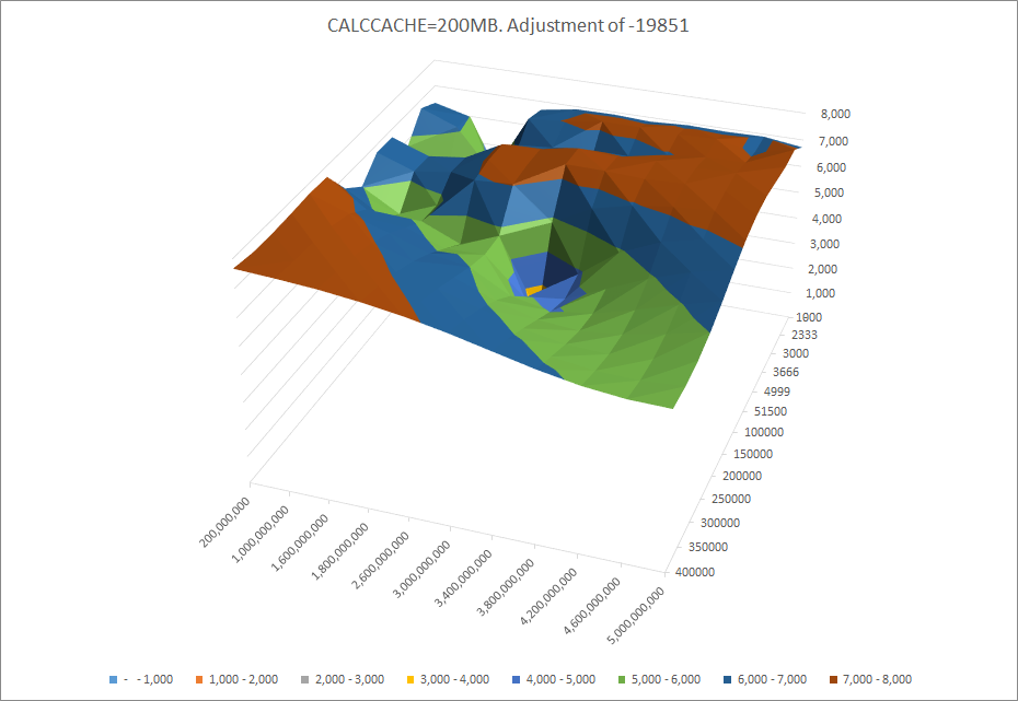
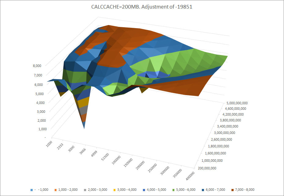
Once we or self tuning algorithm finished running additional tests we may want to present data in a 3D graph again for a larger result set. But how can we do this, if we have missing results for some combinations? Those data points are obtained by the smoothing function, which finds an approximation, based on the surrounding results.

This table shows the new result set with numbers in bold obtained by the smoothing function.

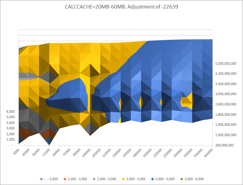
Now you can review the graphs, and identify areas of high performance, or you could simply select configuration with the best performance. In this example we see 2 areas for the maximum calc cache of 200mb.:

Low level commit intervals at high data cache.
High commit interval with low datacache.

Trend

Two areas with higher performance:

Low level commit intervals at high data cache.
High commit interval with low datacache.

LOADCELLSPERSEC=27,231
COMMIT: 5,000.
CALCCACHE: 200MB
DATACACHE: 3,000MB

LOADCELLSPERSEC=27,524
COMMIT: 400,000.
CALCCACHE: 200MB
DATACACHE: 200MB

At the medium size of calc cache between 20 MB and 60MB performance is mostly affected by commit interval.


	Trend Improving performance as commit interval rises. LOADCELLSPERSEC=27,676 COMMIT: 300,000. CALCCACHE: 50MB DATACACHE: 1600MB

And at the low levels of calc cache the the best performance is in isolated area of 3GB data cache, and commit interval of 200,000. This is also a global optimum.

Trend

Isolated areas of high performance around 2-4GB of DATACACHE, and at commit intervals of 125,000 and 200,000.

LOADCELLSPERSEC=27,740
COMMIT: 200,000.
CALCCACHE: 5MB
DATACACHE: 3,000MB

LOADCELLSPERSEC=27588
COMMIT: 125,000.
CALCCACHE: 5MB
DATACACHE: 2,000MB

Now we can move on to finding the optimal number of threads in our calculation.

We define 2 domains: number of CPUs from 1 to 6 and level of the calc cache. We get the best performance at 3 CPUs and at the cacl cache of 5MB.


	Trend The best results are shown for single-threaded calculation for 0.2Mb and 20Mb of CALCCACHE, and for 3 threads at 5Mb of CALCCACHE.

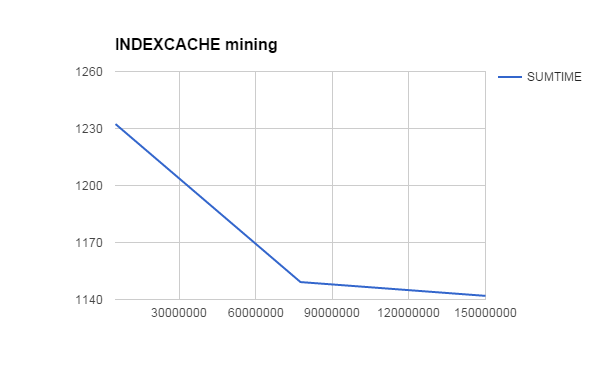
And finally we ran tests to find optimal INDEX cache and compression.

Increasing INDEXCACHE from 50Mb improves performance until INDEXCACHE reaches 75Mb (~30% of index file of 250Mb). Beyond 75Mb increasing INDEXCACHE has little impact.

If you paid attention at the numbers, you could notice that overall, the differences in performance are not huge. The difference between the best and the worst result of domain mining tests is about 30%. But that is after we found best block composition and dimensions ordering. Optimizing those brought the biggest benefit so far.

In terms of caches and commit interval there are some areas that you would want to avoid, but you wouldn’t be able to get improvements of hundreds percents. It is important to know though, since if the requirement is to substantially improve performance, you won't be able to do this by throwing in additional memory and CPUs. You would need to change the design, and only after that those parameters could become relevant. This is something you would want to know before buying new hardware, or simply in order not to waste resources, if performance improvement is not significant.

The counterargument to what i just said about the new hardware could be, well, you run your tests on the old hardware, how do you know that the new hardware with SSD drives for example would not improve performance substantially? And most likely it would. That’s why we also need to run hardware performance monitors at the same time, identify bottlenecks, and analyze data you collect from your tests.